Hack 60. Use Excel to Reorient Access Data

Use Excel's Paste Special Transpose feature to turn data on its ear.

Here's an easy way to change columns to rows (or rows to columns; I guess it all depends on how you look at it). Figure 7-6 shows a table filled with some data. The table contains 8 fields and 100 rows of data.

Figure 7-6. Eight columns of data in a table

Perhaps your user wants to view the data so that each person's record is displayed vertically, which isn't an uncommon request with Excel users. This hack shows how to do just that: put this data in Excel, but turn it sideways.

First, select all the data in the Access table; then, pop over to an open Excel workbook. Find an empty worksheet, and paste the data. Note that for this example, I have purposely pasted the data in row 12. You will see why in a moment. Figure 7-7 shows how the data landed in Excel.

Figure 7-7. Access data pasted in Excel

Upon being pasted, the data is in a selected state. That's great! Just leave it as is, but if you lose the selection, just select it again. The next step is to copy the data, by either selecting Edit Copy or pressing Ctrl-C. Copying the data is a necessary step. It might seem that the data is already on the clipboard. It is, but not in the way we need; therefore, the extra copy from within Excel is necessary.

Now that the data is copied in an Excel format, click in cell A1. This removes the selected state from the data, but that's okay at this point. In fact for the next step, the data must be deselected, and a single cell must be active.

Use the Edit Paste Special menu to open the Paste Special dialog box, as shown in Figure 7-8.

Figure 7-8. The Paste Special dialog box

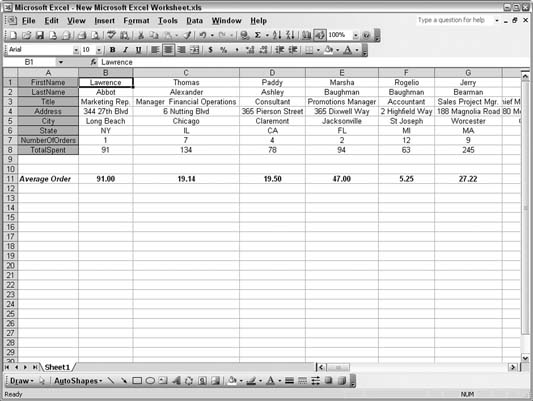
There are few things to note in Figure 7-8. As already noted, the data is deselected. Cell A1 is the active cell. The Paste Special dialog will paste the copied data in the next operation, but the critical point is that the Transpose box is checked. This checkbox is near the bottom of the dialog box.

Clicking the OK button completes the process. Figure 7-9 shows how the data sits at the top of the worksheet. Earlier, I made the first paste in row 12 to give enough room for the second paste. We already knew there were eight fields of data, and now they occupy eight worksheet rows. Although not visible in Figure 7-9, the data goes 100 columns to the right.

The data in the first paste is no longer needed, so you can delete it. A few formatting changes will make the data presentable and ready for work. Figure 7-10 shows how the data looks after a facelift and how analysis is already being run on the data.