A graph is a collection of V vertices and E (directed or undirected) edges that join the vertices into pairs (see section 6.3). This abstraction reflects a very common pattern; the number of systems and relationships that can be modeled by a graph is huge. An example of a graph that will be called G1 in this chapter is shown in Figure 10.1.

Figure 10.1
G1 has two components: subgraphs G11 with vertices {S-P-R-E-A-D-I-N-G} and G12 with vertices {O-U-T}. A component is a maximal subgraph having a sequence of edges connecting any two vertices in it.
A sequence of edges connecting two vertices is a path, but the sequence of vertices encountered as endpoints of the edges defines the same path. A simple path is one that repeats no vertex. For example, (S,A,P) specifies a simple path from S to P but (S,A,I,G,D,R,A,P) is not simple.
A cycle is a path that is simple except that the first and last vertices are the same. For example, (R,D,G,R) is a cycle.
A graph with no cycles is a tree. A collection of trees is a forest. Every connected component of a graph contains spanning trees, trees that contain every vertex in the graph. One spanning forest of G1 is shown in Figure 10.2.
Edges may have a cost (distance, weight) associated with them, as in a model of an airline-route system. A minimal spanning tree is one with the minimal total cost of the included edges. With weighted edges, pairs of edges joined by paths have a shortest path--of minimal total weight. Neither minimal spanning trees nor shortest paths are unique, and the latter may not lie in the former.
Exercise E10.1 is appropriate at this point.
If two vertices are joined by an edge, they are adjacent. Graphs in which every pair of vertices is adjacent are complete. Graphs that approach completeness are dense. Those with few edges are sparse. As a working definition, graphs for which E is much closer to V than to V2 are sparse.
A subgraph of a graph is biconnected if the removal of any one vertex leaves it connected.
Exercise E10.2 is appropriate at this point.
Given a representation of a graph, some of the processes that are of common interest are:
Traverse it in one of a variety of ways, visiting every node.
Determine its components.
Determine whether there is a path between vertex v1 and vertex v2.
Find a spanning tree in it.
Find out if the graph contains a cycle.
Determine its biconnected components.
Also of interest for weighted graphs:
Find a minimal spanning tree in it.
Find the shortest path between two vertices.
The efficiency of these operations depends on the data structure used to represent a graph as well as the algorithm used to traverse it.
10.2 The Priority - Queue Traverse of a Graph
10.3 Applications of Priority-Queue Traverses
10.4 Traverses of Weighted Graphs
A graph can be represented by itself in the sense that every vertex can be represented as a node linked to all adjacent vertices. For an arbitrary graph of N vertices, N -- 1 link-fields would be needed in the nodes. The vertices of a graph may have a limited degree (number of edges to adjacent vertices). A graph of degree 2 or 3 or 4 could reasonably be represented as itself and a general visitation algorithm such as those of section 7.7 or Part II, section M, applied to traverse its components. Determination of some of its attributes would be difficult, however.
As usual with data structures, a graph representation may be either endogenous or exogenous. Processing is simplified if it is assumed that the structure is exogenous, and access to the information that would appear in a vertex is reduced to an index, 1 . . . N. The index can be used as the argument of a function that maps it to the corresponding information, including a node identifier. In this chapter, Tag(k) is taken to be the identifier of vertex k. In the other direction, if id is the identifier of a vertex, Index(id) is the corresponding index. Hence Index(Tag(k)) = k and Tag(Index(id)) = id.
We assume here that the raw data concerning vertices and the edges connecting them are available from a file, perhaps the system input file, and that the maps Index and Tag can be created as the data is read. We assume that the number of vertices V and the number of edges E are also known. In practice, sentinel values or End-of-File flags may be used during input, and the entries counted. The function Index in practice may be a search for an index field in a node, just the application of a Pascal ORD function, a search through a sorted table of identifiers, or several other possibilities.
The timing estimates applied to the algorithms of this chapter assume that Index and Tag are O(1).
The efficiency of the representation of a graph depends on whether it is sparse or dense and which algorithms are applied to that representation.
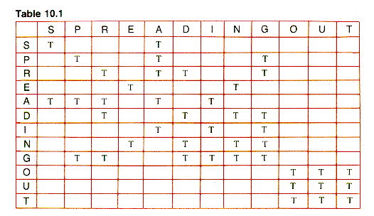
One common representation (introduced in section 6.3) is the adjacency matrix. In simple form, it is a Boolean matrix with TRUE entries in row i and column j iff vertices i and j are adjacent. (Variations are a binary matrix using 1's and 0's or a REAL matrix with values representing weights.) For some applications, it is convenient to set the main diagonal entries (at (1,1),(2,2), . . . ) to TRUE, and that is assumed in this chapter for unweighted graphs. The results for G1 are shown in Table 10.1, where T is used for TRUE and FALSE entries are blank.
If a graph is dense, an adjacency matrix representation is viable. Almost any algorithm applied to the structure will examine the V2 entries in the matrix, but a dense graph has that order of edges to examine anyway.
Given V, E, and Index, the Create procedure for an adjacency-matrix representation is:
For sparse graphs, a common representation of a graph is the adjacency-list, not to be confused with the circular-list structure applied to sparse matrices in section 6.3. In its abstract form, the adjacency listing for G1 is:
Exercise E10.3 is appropriate at this point.
The adjacency-list structure used here is an array of pointers to linear lists, one pointer per vertex. The list associated with a vertex pointer contains nodes that represent edges. The nodes of such a list contain the index of the vertex that the edge connects to its header vertex. For example, the (partial) list
is actually represented by Figure 10.3 if S,P,R, . . .,T are nodes 1,2, . . .,12.
Note: The link structure L can also be a linked list of header nodes, and the adjacency node values are then pointers to the headers.
Creation of the adjacency list with the simple structure illustrated above is done by:
One way to traverse a graph is:
PQT: repeat
1. Process some vertex, k.
2. Put all vertices adjacent to k "on hold"; that is, place them in a holding structure and mark them to be in the state HELD, giving them a priority value. The other possible states for vertices are DONE (processed) and UNSEEN (not adjacent to any DONE vertex).
3. Choose a vertex from the holding structure as the new k.
until all vertices are in the stale DONE.
In step 2 of PQT, a vertex m adjacent to k may already be in state HELD, in which case an algorithm based on PQT may or may not change the priority of m.
A priority queue, section 8.6.2, is the natural holding structure for such a traverse. In some algorithms derived from PQT, the priority-queue acts as a stack or as a queue, and should be replaced by the simpler and more efficient structure. In some applications of PQT, an unordered list may be an efficient representation of the holding structure, but it is used as a priority queue.
When vertices are held in a stack, step 3 of PQT chooses the most recently held vertex. However, the priority of vertices adjacent to it are (re)determined, even if they are already in the priority queue. In effect, they are moved to the top of the stack when reencountered. (The priority of vertices in state HELD are updated during the traverse.) The result of using a stack in this sense is depth-first-search (dfs). Starting at S in G1:
At this point, all vertices reachable from S have been processed -- a component has been discovered, and a new start must be made:
When vertices are held in a queue, step 3 of PQT chooses the longest-held vertex. The result is a breadth-first-search (bfs). Starting at S for G1:
At this point, all vertices reachable from S have been processed -- a component has been discovered, and a new start must be made:
A quite different trse results when the graph edges are weighted, and the weights are used for priorities. A weighting of the edges of G1 is shown in Figure 10.4.
Since the weights are of edges, not vertices, the "weight" of a HELD vertex is continually updated to be the lowest weight of any edge connecting it to a vertex that is in state DONE. For W1, starting at S:
At this point, all vertices reachable from S have been processed -- a component has been discovered, and a new start must be made:
Note: The order in which vertices of a graph are processed is affected by their entry order, the vertex at which the search begins, the process of insertion into an adjacency-list, and perhaps some details of the implementation of PQT. There is not one breadth-first or depth-first search, but there is a family of them.
A number of refinements may be made to PQT in implementation, and they involve several variables and lists. For sparse graphs supported on an adjacency-list with link-header list L, a traverse uses the following:
Unseen is the state value of a vertex not yet encountered in a traverse. It is treated here as an integer larger than any other priority.
Root is a state value attained only by the first vertex of a component--one that is processed before any vertex to which it is adjacent is processed. Zero is usually used for the value of Root.
T counts the number of vertices removed from state UNSEEN--hence, the number of vertices that have been encountered in the traverse at any point in the traverse.
PQ[1 . . V] is an indirect priority queue in which low values have a high priority. It contains indices of vertices. It does not appear explicitly in the algorithm but is used by the priority-queue operators. All vertices are initially placed in PQ, with priority Unseen. The value Unseen is chosen to be greater than the priority of any HELD or DONE vertex. Vertices are removed one at a time with function Remove, as they are processed.
Priority is a variable calculated to sequence the removals from PQ and hence its definition varies from one application to another. It may be set to T for breadth-first search, V -- T for depth-first search, or an edge-weight to find a minimum spanning tree.
OnPQ[1 . . V] is a Boolean list for which OnPQ[k] is TRUE if the kth vertex is still in PQ.
State[1 . . V] contains the priorities of the vertices in PQ. When changed, the values in State are set to a Priority value.
L[1. . V] is the list of adjacency-list headers.
Remove returns and deletes the front value of PQ.
With these tools an adjacency-list traverse is:
Processes 0,1,2,3, and 4 are null or simple or elaborate, depending on the application. If they are all null, then the traverse leaves no trace of its passage and builds no structures suitable for further processing in an application; hence, their use is precisely to build a legacy.
An adjacency matrix form of this procedure, DensePQT, can be constructed by simply replacing the while loop with:
This section describes information that is easily extracted during a priority-queue traverse of a graph.
10.3.2 Path-Connections and Components
The list of vertices in the sequence in which they are processed (in PROCESS1) is the process sequence. The entry for the root of a component in the process sequence is negated to make component detection easier. The list is kept in Done[l . . V] and generated by the inclusions:
The list that specifies at what position in the sequence a vertex is processed is the process map. In effect, it is an inverse of (the absolute value of) Done and kept in WhenDone[1 . . V]. WhenDone[k] = c iff |Done[c]| = k. WhenDone is generated simply by changing the PROCESS1 generation of Done to:
A vertex k that determines the final priority of a vertex m is its Parent, kept in Parent[1 . . V]. Parenting data is gathered by:
A vertex that pulls the vertex m into the HELD state from the UNSEEN state is the earliest-processed vertex adjacent to m and is called its ancestor. The list Ancestor[1. . V] can be generated with:
The data-collection lists Done, WhenDone, Parent, and Ancestor are all generated for essentially no execution-time cost with O(1) operations. However, they do not directly answer the questions about graphs mentioned at the beginning of this chapter and certainly they do not represent the most convenient form for working with components, paths, and spanning trees. Mining the ore they represent is the subject of the subsections that follow.
Note: Almost any application of the preceding data-acquisition lists can be done more succinctly and often more efficiently by incorporating their ultimate use into the traverse itself. The advantage of using them as a standard data-collection format is just that--a system one can come to know and understand and apply quickly.
A trace of the generation of the data-lists by a dfs on G1, starting at S is:
The resulting values are summarized in Table 10.2.
Program PG10.1 is appropriate at this point.
The progress of a traverse may be printed (or listed on a file) with:
Components may be separated in the listing with a marker (such as an End-of-Line) by moving the Write below the test for Unseen and adding:
PROCESS2: Write(EOLN)
This separation is possible because, if the vertex pulled from PQ is in state UNSEEN, it is not reachable from any previously processed vertex and must be in a different component.
Because Remove is O(1n V) when PQ is implemented as a heap, and every edge and every vertex is examined, traversal time for SparsePQT is seen to be O((E + V) ln V). This can be improved to O(E + V) when PQ is replaced by a stack (for dfs) or a queue (for bfs). For DensePQT the corresponding times are O(V2 ln V) and O(V2).
A linear scan of Done yields sets of vertices in the same component, separated by root vertices with negative entries. In a computing system that supports set variables and manages them efficiently, the component data may be shifted into sets during a linear scan for further processing.
If Done itself is to be used to decide whether two vertices are path-connected (in the same component), it is necessary to scan the component that contains one of them. If WhenDone[k1] = c1 and WhenDone[k2] = c2, then k1 and k2 are in the same component iff there is no negative entry between c1 and c2 in Done. This is an O(V) operation for each pair of interest. If it is to be repeated, a scan can be used to build a list of component-completion times, a binary search used to place c1 between two of them, and a quick check used to see if c2 lies between the same pair of component-completion times.
The union-find operations of section 9.7 can be applied to Parent to build set structures within which the search for a common root node efficiently answers the question of whether two vertices are in the same component.
An approach more efficient than union-find structures uses Done as a guide to construct fully collapsed component sets. The procedure MakeSet that follows points all of the vertices to the root node of their component, which has an index that is the current value of SetLink.
The Boolean expression for path connection is then:
Note: MakeSet works for T and V -- T priorities because with their use, root nodes are processed before other nodes in any component. It will not suffice otherwise.
The root nodes in Set are self-referencing, as an alternative to root indices of value 0.
The logic of MakeSet can be incorporated into SparsePRT (or DensePQT) by:
If Done is not needed for any other purpose, it may be dispensed with:
Exercise E10.4 is appropriate at this point.
The data in Parent determines a spanning forest, but the links point from child to parent, in the wrong direction for most tree processing. A treeform that can be traversed from root to leaf is an adjacency-list that omits links extraneous to the forest. Figure 10.5 shows the dfs traverse of G1 beginning at S.
Such a forest can be formed from a linear scan of Parent:
This process can be included in SparsePQT (or DensePQT) by:
The data in Ancestor also determine a spanning forest. It may be generated directly in processes 0, 2, and 3 without the use of the list Ancestor.
Exercise E10.5, problem P10.1, and program PG10.2 are appropriate at this point.
A connected graph G has a cycle iff a spanning tree does not contain all of the edges of G. An extra edge (v1,v2) provides a path (not in the tree) between v1 and v2; and, together with the connecting path through the tree, it forms a cycle. A graph has no edges that connect trees in its spanning forest, and so any edge not in the forest forms a cycle within a component.
For any edge (k,m) one vertex say m, is processed later than the other and so is encountered in the adjacency loop of the other. An extra edge can be detected as an adjacency of m to a vertex n where n is processed prior to k. In simplest terms, when this occurs, OnPQ[m] is TRUE and State[m]
All cycles will be detected (and so could be counted or otherwise noted) because all edges are examined during the traverse.
An articulation point of a graph is a vertex with the property that, if it is removed, the remaining subgraph has more components than the original. All connecting paths between some parts of the graph and others must pass through it. The articulation points in the graph G2 of Figure 10.6 are A, B, and C.
A biconnected graph is one where every pair of vertices is connected by at least two disjoint paths, so it has no articulation point through which all of the paths between some pair of vertices must pass. If the edge (E,F) is added to G2 to form G3, then G3 is biconnected.
Biconnected components (maximal biconnected subgraphs) are not disjoint, in contrast to (connected) components. For example, G4 in Figure 10.7 has two biconnected components joined by the articulation point K, which lies in both of them.
As a result, a reasonable goal in the exploration of the biconnectivity of a graph is the determination of its articulation points.
The information needed to detect articulation points is implicit in a search tree generated by dfs when used in conjunction with the edges not in the tree--ghost links.
The dfs search forest for G1 by dfs starting at S has four ghost links, dashed in Figure 10.8. The dfs search tree for G2 starting at C has one ghost link, as it must, since there are seven vertices and hence precisely six edges in the spanning tree itself. The seventh edge must be a ghost, as shown in Figure 10.9.
Here C is an articulation point because the entire graph cannot be searched from just one of its children--it is the only link between the subtrees rooted at its children.
Note: All ghost links (edges left out of the dfs spanning tree) connect vertices to their ancestors. If there had been an edge connecting sibling subtrees, it would have been followed during the search of the first subtree to be processed.
As one consequence of this note:
If the root of a dfs search tree for a component has more than one child, it is an articulation point.
This form of articulation point can be detected by a linear pass through either Done (for negative entries) or Parent (for zero entries) or Ancestor (for zero entries) to find component roots. An O( l ) check of Forest detects multiple children for such vertices.
A ghost link, such as (C,F) in T3 (Figure 10.9), forms a cycle. All of the vertices from the ancestor down through the search tree to the parent to the ghost link vertex and back through the ghost link to the ancestor lie in the cycle and hence form a biconnected subgraph. The possible articulation points in this cycle are vertices with children not on the cycle and the ancestor. (The ancestor may be the only bridge between the cycle to that part of the graph higher in the tree.)
If a vertex k has a child that roots a subtree with no ghost links to vertices higher in the tree than k, then removal of k disconnects this subtree from the parent of k (and higher nodes). In general:
A nonroot vertex k is an articulation point iff it has a child that roots a subtree that has no ghost links to vertices higher in the tree than k. (Vertices higher in the tree are necessarily processed earlier.)
We define the minimum completion time (mct) of a collection of vertices {w1, . . ., wm} to be the minimum completion time of their collective ancestors (to which they are connected by either tree links or ghost links).
Suppose that the completion time of vertex p is c. Then c is an upper bound on the mct of each of the subtrees rooted by its children because there is a link or ghost link from p to each child. If any such subtree has an mct of c, p is an articulation point. The union of p and its subtrees has an mct that is the minimum of the subtree mcts and the completion time of the ancestor of p. Children are necessarily completed later than their parents. This suggests a way to search for articulation points:
1. Scan through Done backwards, assigning values to lists UrMin[1 . . V] and UrMax[1 . . V ]. They contain, respectively, the earliest known ancestor completion time and the latest known ancestor completion time of the subtrees rooted by the children of the vertex.
2. Suppose that vertex k is not a component root and its completion time is c. When the scan is complete, if UrMax[k] = c, then k is an articulation point.
3. The entries of Children[0 . . V] are initialized to zero. During the scan Children[k] is incremented whenever one of the children of k is processed. Then a component-root r for which Children[r] > 1 is true is an articulation point.
The resulting procedure is:
Note that UrMax[k] remains 0 for a leaf vertex k. A partial trace of the variables in Articulation from the data-acquisition lists of section 10.3 generated by the dfs search of G1 is shown in Table 10.3.
Completion of this trace and determination of UrMin and UrMax are left for an exercise. However, the last entry shown is sufficient to determine that
and hence vertex 8 is an articulation point.
Exercise E10.6, problem P10.2, and program PG10.3 are appropriate at this point.
The weighted graph W1 of section 10.2 is reproduced as Figure 10.10 for convenience.
Weights are an attribute of edges, but a spanning tree that is to be traversed from vertex to vertex needs to have them attached to the vertices. Vertex weights are determined during the construction of the tree using the following definitions:
DEFINITION: The weight of a vertex in state UNSEEN is Unseen. The weight of a vertex in state HELD is the minimum weight of the edges that connect it to vertices in state DONE. The weight of a vertex in state DONE is the weight with which it exits state HELD.
The fundamental source of a weight is an adjacency-matrix entry or a field p
When vertex m is processed in the adjacency loop of vertex k in SparsePQT, the value of the variable Priority is p
The spanning tree derived from dfs by using weights as described above is a minimal spanning tree, produced by what is known as a greedy method. The crux of a greedy method algorithm is that it makes the best available move based on the information available at any stage of the process. In some situations, and forming a minimal spanning tree is one, a global optimum can be derived by repeatedly using a local optimum--the greedy method.
When the greedy method is implemented with DensePQT, it follows the scheme known as "Prim's Algorithm." An alternate scheme, known as "Kruskal's Algorithm" is to choose edges one at a time, lowest-weight first, rejecting those that would close a cycle if added to the forest. When complete--all vertices are included--there is one spanning tree for each component.
The traditional approach to Kruskal's Algorithm retrieves edges from a sorted list, say Edges [1 . . E]. A heap of edges would do as well but would save no processing time: retrieval of all edges is a sorting process of order (E In E). An edge in the list is taken to be a record e that contains a weight e
When an edge e is used to attach vertex m to a vertex k already in the forest, the process of attachment involves lists already familiar from section 10.3:
The resulting lists can be applied as they were in section 10.3, with minor variations. Parent entries of component roots need to be changed from self-reference to zero for complete conformity. WhenDone[k] is the time at which k is added to the forest, but not necessarily when it is joined into its final component tree.
Figure 10.11 shows some snapshots of the process applied to W1.
At this point, all of the vertices have been chosen; but, as Figure 10.12 shows, the trees of the forest do not represent components of the graph.
Problem P10.3 is appropriate at this point.
The test for cycle generation is a test to see if the two vertices of an edge lie in the same tree. Set will not work as it did in section 10.3.3 because component roots are not identifiable until the process is complete and roots are not necessarily added before their children. Some variation of the Find operation of section 9.7, acting on Set, is needed to test for a common component.
The version of Kruskal's Algorithm presented here examines the vertices of the (greedily) chosen edge. Neither, one, or both are already in the forest: vertex m is in the forest if WhenDone[m]
Program PG10.4 is appropriate at this point.
10.4.1 The Shortest Path Problem
The shortest path problem is to find the path in a weighted graph between two given vertices that has the minimal weight sum of all such paths.
If the weights are all one, bfs will find the shortest path from the starting vertex to all vertices in its component. A bfs search attaches to a component tree all vertices reachable from the root with one edge, then all those reachable with two, and so on.
The minimum spanning tree determination with SparsePQT repeatedly adds the vertex closest to the tree. The shortest path variation is simply to add the vertex closest to the root vertex r from which paths are to be formed. (Its state may be initialized to zero instead of UNSEEN so that it is chosen first.)
Suppose that SparsePQT is used to derive the shortest path. During the traverse, the vertices in state DONE are connected to r by shortest paths. If m is moved into state HELD from state UNSEEN in the adjacency loop of k, the shortest known path from m to r is formed by attachment of m to the tree at k. The total path length to r is the path length from k to r plus the weight of the edge (k,m). If m is already in state HELD, the path from m to k to r may or may not be shorter than the shortest path known prior to the processing of k. The test is simply made by using:
The final path length from r to any k is in list State; the individual edges in the shortest path tree can be derived from list Parent.
A variation for dense graphs, using the adjacency matrix, is to use the list State simply as that: an unordered list. The State entries of vertices not yet in state DONE are negated to distinguish them. The Remove procedure is replaced by a linear scan for the largest negative vertex (closest to zero). When the state of a vertex is changed in the adjacency loop, it is changed to - priority. When a vertex is moved into state DONE, its State entry is complemented to make it positive.
The use of a[k,m] for Priority values yields Prim's Algorithm for the minimal spanning forest, and the use of State[k] + a[k,m] for Priority values yields Dijkstra's Algorithm for the shortest path problem.
Program PG10.5 is appropriate at this point.
Problems of interest in a wide variety of applications include the mathematical model, graph. Graph models have been used for a long time and have accumulated a great deal of nomenclature concerning their paths and cycles. Graphs can be modeled in a program in a number of ways. The two most common structures for representing a graph are the adjacency matrix, most suitable for dense graphs, and the adjaceny list for sparse graphs.
A basic requirement of most algorithms that deal with a graph is a traverse of it, generally to make a search for something. The approach taken here is to describe a very general traversal that can be specialized and perhaps made more efficient for particular uses. It is a priority-queue traverse, PQT. PQT is shown to be general enough to include dfs (depth-first search) and bfs (breadth-first search).
PQT is used to generate data-acquisition lists Parent, Ancestor, Done, and WhenDone. These in turn are used to answer questions about a graph--its cycles, components, paths, spanning forest, and biconnection properties.
The use of edge-weights for priorities in PQT allows it to be used to find minimal spanning trees and shortest paths.
This chapter is formed around a central algorithm. PQT can be specialized, tuned, and expanded as needed. An advantage to this approach is that customizing can be done on familiar grounds, using the programmer's time efficiently.
The reader seeking background material on graphs for this chapter can try any number of finite mathematics texts. They usually include a chapter on graphs and indicate some of the areas of application. A survey of applications at a higher level is [ROBERTS, 1978], which has been supplemented by [ROBERTS, 1984]. Both contain extensive bibliographies.
Numerous books on graph theory are available for the undergraduate level, and the list is growing. The choice is yours. The same is true of books titled Discrete Mathematics.
Graph algorithms are being researched extensively. Several books about graph algorithms exist, and again the list is growing. One such is [EVEN, 1979].
A nice treatment of priority-queue traverses, including recursive versions, is given in [SEDGEWICK, 1983].
A number of graph-algorithm topics not covered in this chapter are relatively accessible. They include those for directed graphs, networks, and matching problems. Both [SEDGEWICK, 1983] and [TARJAN, 1983] have good treatments of these topics.
Exercises immediate applications of the text material
E10.1 Find the smallest graph with more than one minimal spanning tree (mint) and a mint-(shortest-path) pair that have no edges in common.
E10.2 In G1 of section 10.1, determine:
(a) the longest cycle
(b) a spanning forest different from the one illustrated
(c) the largest biconnected subgraph
E10.3 Form the adjacency listing and adjacency matrix for G1 if the nodes are in alphabetical order.
E10.4 Trace the operation of MakeSet on the summary data for G1 given in section 10.3.
E10.5 Draw the spanning tree for G1 that would be produced by MakeForest altered to use Ancestor rather than Parent.
E10.6 Complete the trace of Articulation variables started in section 10.3.5 and determine UrMin and UrMax.
Problems not immediate, but requiring no major extensions of the text material
P10.1 Incorporate the effect of MakeForest (section 10.3.3), using Ancestor rather than Parent, directly into SparsePQT (section 10.2).
P10.2 Design a procedure that uses UrMax and Children to determine and list of articulation points.
P10.3 Change all of the weights w in W1 (section 10.4) to 10 - w and trace the behavior of Kruskal's Algorithm with snapshots.
Programs for trying it yourself
PG10.1 Write a program that will read a file of vertices and edges and display a summary of data-acquisition lists like the one for G1 at the end of section 10.3.
PG10.2 Write a program that determines and displays the spanning forest of a graph. A variation is to use PG10.1 to write files used as input by this program.
PG10.3 Write a program that inputs vertex, edge, and identifier data for graphs and displays components and articulation points. A variation uses the program of PG10.1 to create files used as input for this program.
PG10.4 Write a program that sorts an edge list of a graph and applies Kruskal to it and displays the data-acquisition lists that result from it.
PG10.5 Write a program that uses SparsePQT to determine the shortest paths from a given vertex to all the vertices reachable from it.
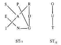
Figure 10.2
10.1 Graph Representation
Table 10.1
procedure CreateAM {O(V2 + E)for i = 1 to V do
for j = 1 to V do
a[i,j]
 FALSE
FALSEnext j
next i
for i = 1 to V do a[i,i]
 TRUE next i
for e = 1 to E do
Read(id1, id2)
i
 Index(id1)
j
 Index(id2)
a[i,j]
 TRUE
TRUEa[j,i]
 TRUE
TRUEnext e
end {CreateAMS : A
P : A G
R : A D G
E : N
A : S P R I
D : R N G
I : A G
N : E D G
G : P R D I N
O : U T
U : O T
T : U O
S : A
P : A G
.
.
.
A : S P R I
.
.
.
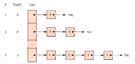
Figure 10.3
procedure CreateAL {O(V + E)for k = 1 to V do
L[k]
 NIL
NILnext k
for e = 1 to E do
Read(id1, id2)
i
 Index(id1)
j
 Index(id2)
NEW(p)
p
 .Value
  j
jp
 .Link
.Link  L[i]
L[i]L[i]
 p
pNEW(p)
p
 .Value
  i
ip
 .Link
.Link  L[j]
L[j]L[j]
 p
pnext e
end {CreateAL10.2 The Priority - Queue Traverse of a Graph
DONE HELD UNSEEN
1. S - PREADINGOUT
2. S A PRE DINGOUT
1. SA PRE DINGOUT
2. SA PRI E D NGOUT
1. SAI PR E D NGOUT
2. SAI PRG E D N OUT
1. SAIG PR E D N OUT
2. SAIG PRDN E OUT
1. SAIGN PRD E OUT
2. SAIGN PRDE OUT
1. SAIGNE PRD OUT
2. SAIGNE PRD OUT
1. SAIGNED PR OUT
2. SAIGNED PR OUT
1. SAIGNEDR P OUT
2. SAIGNEDR P OUT
1. SAIGNEDRP OUT
2. SAIGNEDRP OUT
DONE HELD UNSEEN
1. SAIGNEDRPO UT
2. SAIGNEDRPO UT
1. SAIGNEDRPOT U
2. SAIGNEDRPOT U
1. SAIGNEDRPOTU
2. SAIGNEDRPOTU
DONE HELD UNSEEN
1. S - PREADINGOUT
2. S A PRE DINGOUT
1. SA PRE DINGOUT
2. SA PRI E D NGOUT
1. SAP RI E D NGOUT
2. SAP RIG E D N OUT
1. SAPR IG E D N OUT
2. SAPR IGD E N OUT
1. SAPRI IGD E N OUT
2. 2SAPRI GD E N OUT
1. SAPRIG D E N OUT
2. SAPRIG DN E OUT
1. SAPRIGD N E OUT
2. SAPRIGD N E OUT
1. SAPRIGDN E OUT
2. SAPRIGDN E OUT
1. SAPRIGDNE OUT
2. SAPRIGDNE OUT
DONE HELD UNSEEN
1. SAPRIGDNEO UT
2. SAPRIGDNEO UT
1. SAPRIGDNEOU T
2. SAPRIGDNEOU T
1. SAPRIGDNEOUT
2. SAPRIGDNEOUT
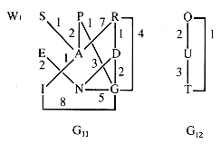
Figure 10.4
DONE HELD UNSEEN
1. S - PREADINGOUT
2. S A PRE DINGOUT
1. SA PRE DINGOUT
2. SA RI E D NGOUT
1. SAI PR E D NGOUT
2. SAI PRG E D N OUT
1. SAIP RG E D N OUT
2. SAIP RG E D N OUT
1. SAIPG R E D N OUT
2. SAIPG RDN E OUT
1. SAIPGD RN E OUT
2. SAIPGD RN E OUT
1. SAIPGDR N E OUT
2. SAIPGDR N E OUT
1. SAIPGDRN E OUT
2. SAIPGDRN E OUT
1. SAIPGDRNE OUT
2. SAIPGDRNE OUT
DONE HELD UNSEEN
1. SAIPGDRNEO UT
2. SAIPGDRNEO UT
1. SAIPGDRNEOT U
2. SAIPGDRNEOT U
1. SAIPGDRNEOTU
2. SAIPGDRNEOTU
procedure SparsePQT
T
 0
0for k = 1 to V do {initializationState[k]
 Unseen
OnPQ[k]
 TRUE
TRUEPROCESS0(k)
next k
CreatePQ {queue all verticesrepeat {retrieve them one by onek
 Remove
OnPQ[k]
 FALSE
FALSEPROCESS1(k)
if State[k] = Unseen {a new component startsthen State[k]
 Root
RootT
 T + 1
T + 1PROCESS2(k)
endif
p
 L[k] {check the adjacency-list
while p
 NIL do
m
 p
p  .Value
if OnPQ[m]
then if State[m] = Unseen
then T
 T + 1
T + 1PROCESS3(k)
endif
if State[m] > Priority
then State[m]
 Priority
PROCESS4(k)
endif
endif
p
 p
p  .Link
.Linkendwhile
until Empty(PQ)
end {SparsePQTfor m = 1 to V do {check the adjacency-listif a[k,m]
then if OnPQ[m]
then T
 T + 1
T + 1PROCESS3(k)
endif
if State[m] > Priority
then State[m]
 Priority
PROCESS4(k)
endif
endif
next m
10.3 Applications of Priority-Queue Traverses
The Process Sequence
:c
 0
0PROCESS1: c
 c + 1
c + 1Done[c]
 k
kPROCESS2: Done[c]
 - Done[c]
The Process Map
PROCESS1: c
 c + 1
c + 1Done[c]
 k
kWhenDone[k]
 c
cThe Parent
PROCESS0 : Parent[k]
 0
0PROCESS4 : Parent[m]
 k
kThe Ancestor
PROCESS0 : Ancestor[k]
 Unseen
PROCESS2 : Ancestor[k]
 O
OPROCESS3 : Ancestor[m]
 k
kS = State A = Ancestor D = Done
Pa = Parent P = Priority W = WhenDone
Tag k m T P S W D A Pa
----------------------------------------
S 1 1 -1 0 0
5 2 10 10 1 1
A 5 2 5 1 1
2 3 9 9 5 5
3 4 8 8 5 5
7 5 7 7 5 5
I 7 3 7 5 5
9 6 6 6
G 9 4 9 7 7
2 6 6 6 5 9
3 6 6 6 5 9
6 7 5 5 9 9
8 8 4 4 9 9
N 8 5 8 9 9
6 8 4 4 9 8
4 9 3 3 8 8
E 4 6 4 8 8
D 6 7 6 9 8
3 9 3 3 5 6
R 3 8 3 5 6
P 2 9 2 5 6
0 10 10 -10 0 0
11 11 1 1 10 10
12 12 0 0 10 10
T 12 11 12 10 10
11 12 0 0 10 12
U 11 12 11 10 12
Table 10.2
Tag[k] k Ancestor[k] Parent[k] WhenDone[k] Done[k]
-------------------------------------------------------
S 1 0 0 1 -1
P 2 5 8 9 5
R 3 5 6 8 7
E 4 8 8 6 9
A 5 1 1 2 8
D 6 9 8 7 4
I 7 5 5 3 6
N 8 9 9 5 3
G 9 7 7 4 2
O 10 0 0 0 -10
U 11 10 12 12 12
T 12 10 10 11 11
10.3.1 Tracking a Traverse
PROCESS1: Write(Tag[k])
10.3.2 Path-Connections and Components
procedure MakeSet {O(V)for c = 1 to V do
if Done [c] > 0
then Set [c]
 SetLink
else SetLink
 - Done [c]
Set [c]
 SetLink
endif
next c
end {MakeSetSet[k1] = Set[k2]
: c
 0
0PROCESS1 : c
 c + 1
c + 1Done[c]
 k
kPROCESS2 : SetLink
 Done[c]
Set[c]
 SetLink
Done[c]
 -- Done[c]
else Set[c]
 SetLink
: c
 0
0PROCESS1 : c
 c + 1
c + 1PROCESS2 : SetLink
 k
kSet[c]
 SetLink
else Set[c]
 SetLink
10.3.3 Spanning Forests
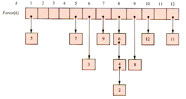
Figure 10.5
procedure MakeForest {O(V)for k = 1 to V do
Forest[k]
 NIL
NILnext k
for k = 1 to V do
p
 Parent[k]
if p
 0
0then NEW(q)
q
 .Value
  k
kq
 .Link
.Link  Forest [p]
  .Link
.LinkForest [p]
 .Link
.Link  q
qendif
next k
end {MakeForestPROCESS0: Parent[k]
 0
0Forest[k]
 NIL
NILPROCESS2: else p
 Parent[k]
NEW(q)
q
 .Value
  k
kq
 .Link
.Link  Forest[p]
  .Link
.LinkForest[p]
 .Link
.Link  q
qPROCESS4: Parent[m]
 k
k10.3.4 Cycle Testing
 Unseen in the adjacency loop of k. The test for a cycle in dfs is then:
PROCESS0: Cycle
 FALSE
FALSEPROCESS3: else Cycle
 TRUE
TRUE10.3.5 Biconnectivity

Figure 10.6

Figure 10.7
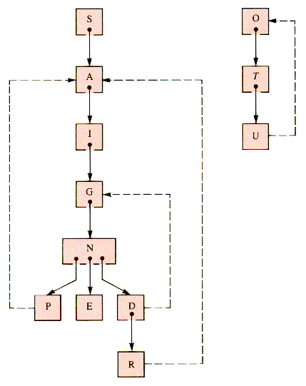
Figure 10.8
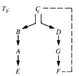
Figure 10.9
procedure Articulation {O(V)Children[O]
 0 {component counter
for k = 1 to V do
Children[k]
 0
0p
 Parent[k]
if p = 0 then p
 k endif
UrMin[k]
 WhenDone[p]
Urmax[k]
 0
0next k
for c = V downto 1 do
k
 |Done[c]|
p
 Parent[k]
Children[p]
 Children[p] + 1
if p
 0
0then a
 Ancestor[k]
t
 WhenDone[a]
if UrMin[k] > t
then Min
 t
telse Min
 UrMin[k]
endif
if Min < UrMin[p]
then UrMin[p]
 Min
Minendif
if Min > UrMax[p]
then UrMax[p]
 Min
Minendif
endif
next c
end {ArticulationTable 10.3
c k p a t Min
12 11 12 10 10 10
11 12 10 10 10 10
10 10 0 - - -
9 2 8 5 2 2
8 3 6 5 2 2
7 6 8 9 4 2
6 4 8 5 5 5
. . . . . .
. . . . . .
. . . . . .
UrMax[8] = 5
10.4 Traverses of Weighted Graphs

Figure 10.10
 .w in an adjacency-list edge node. During a traverse, weights of vertices are stored in State, since they determine priorities. The sum of the final State list is the total weight of a spanning forest.
 .w. (This is the weight of the edge connecting k and m.) It has already been traced for W1 in section 10.2, and construction of the tree itself is covered in section 10.3.3.
 .w, and vertices e
  .a and e
  .b.
.b.procedure Attach(m,k)
c
 c + 1
c + 1WhenDone[m]
 c
cDone
 m
mState[m]
 e
e  .w
.wParent[m]
 k
kSet[m]
 Set[k]
end {Attach
Figure 10.11
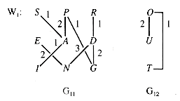
Figure 10.12
 0. If precisely one vertex is in the forest, the other is attached to it. If neither is in the forest, one is attached to the other. If both are in the forest in distinct trees, one is attached to the other; but if they are in the same tree, the edge is rejected:
procedure Kruskal
for k = 1 to V do
Parent[k]
 0
0Set[k]
 k
kWhenDone[k]
 0
0next k
c
 0
0ec
 0
0while ec < E do
ec
 ec + 1
e
 Edges[ec]
if WhenDone[e
 .a] = 0 {e
  .a is not in the forest
then if WhenDone[e
 .b] = 0 {and neither is e
  .b
.bthen Attach(e
 .b,e
.b,e  .b)
.b)endif
Attach(e
 .a,e
.a,e  .b)
.b)else if WhenDone[e
 .b] = 0 {only e
  .a is in the forest
then Attach(e
 .b,e
.b,e  .a)
.a)else if Find(e
 .a)
.a)  Find(e
  .b) {both are in the forest
then Parent[e
 .b]
.b]  e
e  .a {and in distinct trees
Set[e
 .b]
.b]  Set[e
Set[e  .a]
.a]State[e
 .b]
.b]  e
e  .w
.wendif
endif
endif
endwhile
end {Kruskal10.4.1 The Shortest Path Problem
Priority = State[k] + p
 .w
.wSummary
Further Reading
Exercises
Problems
Programs


