


In most HLLs, arrays are automatically available to the programmer, but they are actually created from cells or simpler arrays. When a compiler, an operating system, or an assembler program is written, and when an HLL of limited power is used, arrays are created by the programmer. This chapter serves to isolate properties that characterize arrays as structures and hence organize the building of arrays, and it presents the array structure as a model data structure. A review of the role of variables and arrays in programming is included in section 2.1.
The simplest way to manage data is to place it in a single memory cell and identify that cell with a name. To the machine, the cell identifier is a memory address or the information used to calculate one. In a high-level language, the identifier is the name of a variable. A compiler (or interpreter, or assembler) program creates the bridge from one form of identifier to the other. However the name of a cell is specified, many problems can be solved using only the simple variable as a data structure. Examples of problems natural to simple variable solutions abound in early chapters of elementary programming texts. Many of them are variations of problems like EP2.1 (Example Problem 2.1), EP2.2, EP2.3, EP2.4, and EP2.5, which follow:
EP2.1 Input 10 numbers and print the maximal value of the entries.
EP2.2 Input 10 numbers and print their mean. (The mean of n entries is defined in Part II, section A.4.)
EP2.3 Calculate the nth Fibonacci number, F(n), where F(n) = F(n - 1) + F(n - 2), and F(0) = 1 = F(1).
EP2.4 Given that the average topsoil in this country has a depth of six inches, that each year it is eroding at a rate of l percent of the depth it has that year, and that it will fail to support agriculture at depths below three inches, when does the topsoil depth fall below the critical level?
EP2.5 Input an integer, I, in the range - 32768
Consider a familiar problem like EP2. l . Someone who lacks programming experience might well recognize that ten inputs can form a sequence x1, x2, . . ., x10 and that they can be compared with each other. The direct implementation of these ideas is expressed in such statements as:
This process, of course, is terribly inefficient, particularly if there are 10,000 values instead of 10. Someone with even a little programming experience will recognize that this problem can be solved simply by retaining the largest value so far. (Nearly anyone can solve this problem over a phone, but only programmers seem to recognize how they do it. It is apparently not a trivial task to make the connection between the natural selection process and the use of a single memory location.) A programmer's solution is something like this:
This solution for EP2.1 can be generalized easily to find the maximal value of a sequence of any fixed length. Furthermore, modifications to MaxTen will allow the sequence length to be an input variable, to find out (with a counter) which entry actually determines the final value of the variable Large, how many entries are equal to the final value of Large (with another counter), how many times Large changes value (with a third counter), and so on.
Note that, by isolating the core of the problem, which is finding the largest-so-far value, other questions can be answered as applications of the solution. Had the problem been stated initially as a request for all of the modifications mentioned above, it might have seemed overwhelming. Much of data structures as a subject is concerned with extracting and focusing upon central ideas that can be modified and combined in order to solve specific applications.
Some problems may seem to be simply variations of EP2.1-EP2.5 but actually call for a data structure that is more complex than the simple variable. For example:
EP2.6 Input 10 numbers and display the second-largest value in the set of entry values.
EP2.7 Input 10 numbers and display them in reverse order of entry.
EP2.8 Input 10 numbers and display the negative entries, followed by the others.
EP2.9 Input 10 numbers and display them in nonincreasing order of their magnitude.
EP2.10 Input 10 numbers and count how many of them are larger than their mean.
This list could be much longer, and EP2.6 could be removed from it by clever programming, but problems like EP2.9 permeate a large portion, perhaps most, applications of programming. Example problem EP2.9 is important because data frequently have to be sorted in convenient order. (Can you imagine using a telephone directory where names are arranged according to the date on which a phone was first connected to the system?) Most government policy decisions, such as When can a drug be safely released for sale? and Which vote will mollify the most constituents? are based at some level on statistical calculations like EP2.10 and the calculation of standard deviation (see Part II, section A.4).
Problems EP2.6-EP2. 10 can be solved if all of the data are retained in memory after input, so that more than one pass through the data is possible. The collection as a whole can be identified and retained as a group of storage cells, but it is helpful to give a unique name to each memory cell in the group. A specific cell name is necessary if individual access to the cells is to be provided, but the collection of names might need to be as large as the data set. The solution to this puzzle is built into most high-level languages and is presumed to be familiar to the reader--it is the subscripted variable, or array.
Note: An array with a single subscript is also called a list (usually indicating that it is used as one). It is not, however, a linked list in the sense defined in Chapter 3.
An array has an identifier for an entire group of cells, and (in the simple one-dimensional case) one other variable, the index, is used to select a particular cell within the group. With the usual notation for arrays, one solution to EP2.7 in SUE, with example input and output and a display of the final values of the array x, is:
Among the reasons for studying arrays specifically as data structures, rather than just accepting them as gifts from a compiler, are these:
In some languages, only a limited number of indices is allowed. (Limits of 2 or 7 have been used.) To get around index limitations, a programmer may construct a high-dimensional array within an array of fewer indices. To do so requires a fundamental understanding of how arrays are structured.
It is fairly common to develop high-level, or very high-level, languages for special purposes, such as a "query language" for asking questions about the contents of a data base. Some of the structuring can be patterned after the details of array structure.
Controlling a microprocessor, designing a compiler for a high-level language, tuning the performance of a program, or controlling the interface between a computer and the outside world, often require an understanding of assembler (and machine) languages. Assembler languages leave the formation of arrays and any controls on their misuse to the programmer. Understanding how to use the array structure provided by high-level languages is often not sufficient for assembly language programming.
Data structures are often constructed by a programmer as superstructures imposed on arrays, although the same structures can also be implemented without arrays. Understanding these structures requires that they be distinguished from the array structure itself.
The array is a familiar programming tool. Abstraction of its properties and the operations needed to manage it provide a model that will be applied to unfamiliar structures in this text.
With these motivations in mind, we turn to study what makes an array with a single index the creature that it is.
There is usually an advantage in thinking of an array as a geometrical sequence of adjacent cells, as depicted in Figure 2.1. For ease of discussion, such an arrangement will be called an LSC, for Linear Sequence of Cells.
Actually, from the view of the array user, it does not matter where the memory cells of an array are located, given that the indices provide random access to them: the user must be able to access the cells in any order merely by specifying the name of the array and the correct index. That the individual cells may be jumbled or scattered in memory does not matter so long as the compiler is provided with a map of where the cells are and uses the index as a pointer to the correct one. Of course, cells are often arranged in storage as an LSC; but, on a magnetic drum or disk, for example, faster access may be provided by a different arrangement.
A map from an LSC to physical storage is usually provided by an operating system, which manages fundamental system resources. With such a map in hand, a compiler-writer can treat an array as an LSC, whether or not that is the geometry of the physical storage cells involved. The LSC becomes a logical abstraction for data-handling: a data structure.
When a multidimensional array is declared and used in an HLL, a compiler provides maps and operations that are invoked by statements in the HLL. The maps are needed to convert an array reference to a storage address. For example, suppose that an array is declared as a[0 . . 7, - 1 . . 2,2 . . 4] and managed by a compiler as an LSC occupying memory cells 27, 28, . . ., 122. Then a[5,0,3] is somewhere specific in the sequence of cells, and the collection of such somewheres is a required map. Such maps are also used when programming in assembly language and other situations, and they are the subject of section 2.3.
Maps from one structure to another are invoked by operations described by program statements. In the case of arrays and LSCs, the operations are relatively simple, but they are general enough to apply to the declaration and use of any array that is legitimate in the language being translated. They are even more general than that: the operations CREATE, STORE, and RETRIEVE are needed whenever arrays are used. Their implementation differs from one application to another and is intimately tied to storage maps. The operations essential for array management are derived below as the kernel of a set of general management features that apply to other data structures as well: activation, viability, assignment, retrieval, and location.
Arrays do not spring into existence simply because they are mentioned (although BASIC allows them to do so to a limited extent). Storage must be allocated for them, and in most languages the amount allocated never changes. (SNOBOL provides an exception.) Array allocation is static--once done, it cannot be changed by the program. Activation of those arrays that are supported by a language is done, for example, with a DIM statement in BASIC and a VAR declaration in Pascal. These creation statements also provide information needed to access individual cells of the array--given the location of a[0], where is a[3]? Sometimes, activation must be programmed because the required array features are missing (more indices in BASIC; any array in an assembler language).
The general activation operation is called CREATE, and so is the analogous operation for other data structures. (The first example in the book of a CREATE operation that is not simply a language declaration is based on arrays and is found in section 2.5.)
Activation of an array does not necessarily imply that it has been initialized to a standard value (although it may be in some languages). Strict control of operations can be provided by making retrieval from an uninitialized memory cell illegal. Usually, programs are allowed to retrieve unchecked garbage instead, because the overhead required to make such checks is considered to be too high.
The ability to copy information into the cell of index i of array a is commonly provided in at least two forms:
The general operation will be written STORE(a,i,x) or simply STORE(i,x). Hence STORE(Grade,3,85) has the effect of
The ability to copy information from the cell of index i is provided in at least two forms:
The general operation will be written RETRIEVE(a,i) or simply RETRIEVE(i). Hence RETRIEVE(Grade,3) immediately after the STORE example above will retrieve the value 85.
Retrieval and assignment operations depend upon the ability to locate a specified cell within the array structure. The array index provides direct access to the cell because it determines an absolute memory address. How it does so will be explained in section 2.3. The location of a cell within other structures is not always so direct.
In summary:
An instance of the structure ARRAY is operated on by CREATE, STORE, and RETRIEVE.
Any cell in an array can be accessed by STORE and RETRIEVE through the use of its index.
An array is static in the sense that no cells can be inserted or deleted from it by an operation.
There is usually no check on validity of the values in an array.
Finally, note that CREATE, STORE, and RETRIEVE are implicit rather than explicit in high-level languages, but their service is provided.
STORE and RETRIEVE: it is the mapping of an index to a unique memory location for each possible in-bounds index. This map is needed to build multidimensional arrays from those with fewer dimensions. Even in the one-dimensional case a map is required, because the address of an array cell and its index are not identical--they are just in one-to-one correspondence. In many languages, array indices may lie in a range that does not begin with zero or one: a[L . . U] is to mean that storage is allocated for a[L],a[L + 1], . . .,a[U]. There are U - L + 1 legal (in-bounds) indices in this case.
Note: In some languages, such as Pascal, memory cells in an array may be specified by any values that form an ordinal sequence. For example, a[Red . . Violet] may mean that Red, Orange, Yellow, Green, Blue, and Violet follow in order, as indices. In effect, they represent indices 0,1,2,3,4, and 5. An auxiliary map is used by the compiler to preprocess the names of colors in order to bring about this effect, but the essential coorespondence is still the map of [0 . . 5] onto six memory addresses.
Suppose that the absolute address of a[L] is
(The address
However, this map itself provides no check for an out-of-bounds address. To make such a check requires a procedure or perhaps some variation of the following:
With the use of this function, if the declaration is a[1 . . 10] and the storage is linear, then a[7] has the address Alpha + 6, and a[- 1] is out of bounds. If the declaration is a[- 5 . . 4], then (the same) 10 memory cells are allocated, but a[7] is out of bounds, and a[- 1] has the address:
If two indices are allowed, then the structure may be thought of as a table, arranged in rows and columns, such as in Figure 2.2.
Each pair of indices specifies a row and a column. Usually a[2,3] is thought of as the cross-hatched square in Figure 2.2--row 2, column 3. However, as long as a program is consistent about storing and retrieving from a table, the choice makes no difference at the program level. The picture is merely an aid to the programmer. In some languages, however, a table can be manipulated as a unit, even for input and output. Then it matters whether or not Read(a) is expecting the input in the order row1, row2, . . . or in the order column1, column2, . . . . That is still a programming issue. The structural issue is how to arrange the data in successive addresses Alpha, Alpha + 1, . . . so that the two indices specify a unique memory cell. The two common arrangements are shown in Figure 2.3.
Note: Most versions of BASIC use the row-major scheme, and FORTRAN uses colunm-major storage.
When a table is to be arranged in a linear pattern as is Figure 2.3 (or in a one-dimensional array), the map from an index-pair to an address (or to a single index) is designed to work for only one of these schemes. Figure 2.4 depicts the two common storage arrangements.
Consider the declaration a[1 . . 3,1 . . 4], and assume that a is stored in row-major order. To get to a[2,3], for example, it is necessary to count past row 1 and then choose the third item in row 2. Since there are four items in row 1, the address of a[2,3] is:
Note that the factor of 4 comes from the number of columns in each row.
More generally, for a[1 . . U1,1 . . U2]. the row-major address of a[i,j] would be:
Generalizing further, for a[L1 . . U1,L2 . . U2], the address of a[i,j] would be:
Similar calculations for the column-major scheme are left to the exercises.
The general row-major storage scheme tor a table is pictured in Figure 2.5.
In order to picture the storage layout for three indices i1, i2, and i3 in row-major (or in column-major order), it is necessary to generalize the meaning of "row-major" (or of "column-major"). Row-major storage of an array is normally taken to mean the following if the array is stored linearly:
As addresses increase from the initial value Alpha toward the last address, the first index changes most slowly, and the last index changes most rapidly.
For the declaration: a[1 . . U1,1 . . U2,1 . . U3], the indices change like this:
As a consequence, the last two indices define a table, one selected by the first index, as shown in Figure 2.6.
The front face F is simply the table defined by i2, and i3 when i1, is fixed at 1.
For the most general declaration of a three-dimensional array a, lower bounds Li replace 1, and the address calculation for a[i1,i2,i3] involves counting past (i1, - L1) tables and then locating a spot within table (i, - L1). There are (U2 - L2 + 1)(U3 - L3 + 1) cells in each table that is passed, hence:
For the n-dimensional case, let sk = Uk - Lk + 1, the number of indices in the range of ik. Then:
Suppose, for example, that we wish to find the address of a[0,0,0,0] in an array declared as: a[ - 4 . . 3,0 . . 4, - 5 . . 5, - 2 . . 6]. Then S1 = 8, S2 = 5, S3 = 11, and s4 = 9. The resulting address is:
Section 2.6 contains an application of the unfolding of many dimensions into one.
Exercises E2.1-E2.5 are appropriate at this point.
Jon Bentley's column "Programming Pearls" in the May 1984 ACM Communications contains an array storage scheme that differs from the usual one for a good reason--it saves a valuable resource. Saved is the storage space that can be wasted when a table is sparse--meaning that most of the entries are the same, usually zero. From the standpoint of information retrieval, only two things are necessary: storing the table entries that are not zero (nonstandard) and detecting a zero entry in some way. The structure developed in this section that does these two things follows Bentley's solution to storing a table in less space than is required by the maps of section 2.3.
Suppose that a map is contained in a grid of NR by NC points that include some fixed number, NI, of items of interest--it is static. The items of interest might be the number of finches in the bird sanctuaries on a state grid, or nuclear reactors on a world grid, or sections containing wheat-rust on a satellite image. There are NR X NC grid points and NI may be much less than that. (In Bentley's problem, NI was 2000, NR was 150, NC was 200, and hence NR X NC was 30,000.) By comparison, there are about 200,000 controlled points on a television screen, and over half a million in the input-output table that describes the United States economy. The resolution provided by the human eye would allow even more points of interest on a large road map of Nevada--but they aren't there. Clearly, storage of all points in a table can be very wasteful of space, and the space may not even be available. In examples of this sort, the data that are likely to be provided for the location of a value are two coordinates--row and column.
The core of this problem is twofold:
1. Many fewer than NR X NC items occupy that much storage in the standard row-major (or column-major) map of an array, and the number of items does not change.
2. The row-and-column format is natural to the problem and provided as the input data for the search for a value in the structure.
The core of a solution is to provide maps from row-and-column data into a compact memory space so that it appears to a user to be a standard table. This approach saves the storage resource and preserves ease-of-use. The user's time, effort, and comfort are themselves important resources.
One scheme for packing the nonzero entries of a table T (illustrated in Figure 2.7) is to store only the nonzero entries and associate them with their row index. Figure 2.7 can be reduced to Figure 2.8. In Figure 2.9 the entries and their rows are stacked together in arrays Value and Row, and a map FirstInCol[1 . . NC + 1] provides the index in Row of the first nonzero row in each column of T. The extra column, 6, and its value NI + 1 = 9 is added to provide a sentinel for Retrieve. The resulting structure is SST (for Sparse and Static Table).
If it is assumed that the values and the indices require one word of storage each, conventional table storage requires NR X NC words of storage. The conventional RETRIEVE operation is O(1), and initialization of the structure requires NI STORE operations. A crucial point to be noticed is that NI can be changed with O(1) STORE operations in the conventional scheme.
Part of the price of the compactness of SST is that assignment of a zero to a cell in the structure or insertion of a nonzero value to a cell not represented in the structure would amount to deletion or insertion of a cell. SST just does not provide for this flexibility.
With the same assumptions, SST requires NI words for Value, NI words for Row, and NC + 1 words for FirstlnCol, a total of 2 X NI + NC + 1 words instead of NR X NC words. The RETRIEVE operation becomes:
This is an O(NI) operation because most of the entries could be in a single column and the for-loop would then iterate up to NI times. If table entries are randomly located, the expected number of entries to be searched is NI/NC. (See section 1.3.2.) The search for the row index could be speeded up by using a binary search as discussed in section 8.3 in the sense of making the search for the row an O(In NI) operation. This apparent speedup is misleading, however, because the overhead required to set up and carry out the search is more than would be needed in the linear search above for the small number of row indices expected per column.
This back-of-the-envelope analysis shows that SST may save a great deal of storage space at the cost of some processing time. It is probably not suitable unless the table is sparse with the entries shared fairly evenly by the columns. The trade of processing time for storage is not uncommon, and sometimes the search for either compactness or efficiency will improve both because it promotes thoughtful analysis.
An HLL program that includes SST would create the arrays Value, Row, and FirstInCol simply by declaration. That does not perform CREATE for SST, however, because SST is a data structure that is shaped by its values and reasonably includes those pairs of indices [i,j] that denote nonzero entries. Hence CREATE should include initialization of the supporting arrays.
Suppose that the information for SST is available as a sequence of triplets (i,j,v) representing row i, column j, and value v, and is sorted by column and by row within each column. Then CREATE is both supporting-array declarations and the assignment of values to them.
The initialization procedure illustrates a theme that occurs for other data structures: the care needed to deal with special cases. In the general case, when a row i, column j, and value v are retrieved from an input file, a suitable procedure response is, for the right Dexi:
However, column j of the input triplet may be the one that follows the column of the previous entry triplet, in which case the above is preceded by (for the right Dexj):
What, however, must be done about missing columns? Examination of Retrieve reveals that if S2 is repeated until j = Dexj, the interplay between the two procedures will generally work. In particular, though, what if the first few or the last few columns are empty? Initialization of Dexj to 0 takes care of an empty leading column and a loop similar to S2 takes care of an empty trailing column.
Finally, the sentinel column NC + 1 can be initialized by simply treating it as the empty last column. The result is:
(The indication O(NI + NC) is one way to point out that this algorithm is either O(NI) or O(NC), whichever is larger.)
The interaction of a data structure and its implementation are illustrated with SST by the fact that if the entry triplets were available sorted by row, then column, the roles of rows and columns would switch: Row and FirstInCol would be replaced by Col and FirstInRow. The structure of SST would not change in any meaningful sense by storing the entries one row at a time--SST is an idea imposed on the underlying arrays by the programmer.
For an application where the number of entries in a table makes it sparse, but that number is not static, there are structures more suitable than SST. They include forms of the sparse matrix of sections 6.4 and 6.5 and Part II, section N, as well as the adjacency list applied in Chapter 10. (But they are less suitable than SST for a static table that is simply to be searched often once it is created.)
The discussion of SST given in this section assumes that the values in the structure are the values of interest. Such a structure is endogenous. It is also possible for the entries in Value to be pointers--indirect references to data external to the structure itself. Such a structure is exogenous. The data structure and the operations on it are little affected by such a change, but the leverage available is large. The data accessed through Value may be bulky and sorted on disk or some other external storage medium in any order. When used as an exogenous structure. SST becomes part of a map or directory to a file of records.
Finally, note that SST is an example of information hiding--the details of the implementation are not important at a user level. A user (program) that acquires a value in row i, column j with Retrieve(i,j) is indifferent to the choice between SST and the standard two-dimensional table format referenced by a particular form of Retrieve. The trade-off between compactness and efficiency and the details of implementation are isolated from functional behavior. At the user level, it is the functional behavior of a structure that needs to be considered in order to use the structure as a tool. The details of its design are distractions at that level. In telegraphic form: SST STILL AN ARRAY.
Exercise E2.6, problem P2.1, and program PG2.1 are appropriate at this point.
It is not always the case that array indices are natural identifiers for items that are to be stored, accessed directly one at a time, and retrieved. Consider the following items:
These items could be maintained in lexicographic order, in which case potato would be item number 10 after all items were placed in the list. With standard algorithms, the RETRIEVE operation would be O(In n) and the STORE operation O(n) if order were maintained as the items were entered. While it is true that STORE and RETRIEVE are O(1) operations for arrays, that is only so if the indices are known and the value in the target of a STORE can be discarded. Without a complete set in hand it cannot be known that potato has index 10 in the sorted list of items.
Because an index integer is not known on the entry of one of the items, it would be helpful if the item itself could be used as a key to index the cell where it will be stored. If, for example, the data-space (the set of all possible data values) were the set of all possible recipe ingredients, the required array would be large, and most of it would be wasted as storage for any one recipe.
A solution would be to convert the keys (the list items, here) into unique integers and use them as array indices. A function that does so is called a hash function, the conversion process is called hashing, and the storage structure is called a hash table or scatter-storage. One such function (not commonly used) is to simply associate integers 1-26 with letters A-Z and add the integers corresponding to the letters of an item together. With this function, HF1, the hashed indices are:
Here is an apparent solution, although an array of 145 cells is needed to store these 12 items. For an arbitrary recipe, 20 or 25 items is quite a lot. With this function, there are 2710 possible keys of no more than 10 characters, and the maximum value of HF1 is only 260. The number of possible ingredients, named in English, is several thousand, many of which will have the same HF1 values.
Schemes to restrict the range of the function, like using HF1 (Item) MOD 25, creates the same problem that arises when just one more item is added to this list: broth. HF1(broth) = 63 = HF1(olive). This is called a collision, and collisions are inevitable if a hash table is to be reasonably space-efficient.
Computer scientists have spent much time exploring how to deal with collisions and juggle the space and time efficiency of hash tables because the utility of hashing is not confined to storing recipe ingredients. Hashing should be considered when any large collection of items is to be stored and retrieved efficiently from a small space.
A discussion of hash tables, confined to the use of array support for them, is to be found in Part II, section B. A supplement to the discussion there is found in Part II, section L, and may be read after other support structures have been introduced.
Many things have a natural dimensionality; they are most easily associated with one or two or some number of indices. However, they do not have to be modeled according to their natural dimensionality. Two-dimensional slices can be used to describe three-dimensional objects. Cross-sections of the atmosphere in a weather model or of a person in a CAT-scan can be used to store essentially three-dimensional information. Sometimes three dimensions can be usefully projected into a single pair of dimensions, as in a contour map.
In the other direction, an indexed set of essentially planar structures can be managed with three indices, forming a three-dimensional data structure. Examples include a sequence of board configurations tor almost any board game, an item-count table for each of a family of warehouses. or a set of crossword puzzles.
The success of these dimension changes, however, lies in the fact that they are reversible--it is possible to devise a picture of natural dimension from the data format. On balance, if a programmer thinks most easily and clearly about a problem when it is portrayed as three-dimensional (or two-dimensional or five-dimensional), then it should be programmed in its natural form. This is not simply information-hiding, but information-packaging.
In this section, a game is used as the model of a system that has a natural dimensionality. Games, it should be noted, serve as models for many things because they can be designed to eliminate extraneous concerns.
Suppose that a program is written to monitor (or to play) three-dimensional tic-tac-toe. The rules of the game and its interaction with users are important parts of the program design, but so is the management of a three-dimensional array. Assume that the language L in which the program is written does not allow three indices, and so the board array, B, needs to be unfolded into a one-dimensional array, Stretch. Suppose that the natural three-dimensional array would be declared as
in a language which allowed such a thing. The array B can be used to think about the design of the program, but the program will actually be implemented with Stretch[1 . . 27].
One way to organize the unfolding of B into Stretch is to develop procedures Create, Store, and Retrieve, which handle the index map from three indices to one, and then rely on the language L for the versions of the CREATE, STORE, and RETRIEVE operations that manage the array Stretch. Create, Store, and Retrieve can then be called upon by the rest of the program, much as though the language L did implement three-dimensional arrays. A clean treatment of that management allows the programmer to focus on aspects of the program other than index calculations.
In most languages, Create must be handled by the programmer, in the sense that Stretch must be declared with sufficient storage to hold B. The array Stretch probably should not be declared with any extra cells, simply as a debugging safeguard.
If Retrieve is implemented as a function with three parameters, then
may be used naturally in place of:
A simple version of Retrieve that does no out-of-bounds checks of i, j, and k is:
This can be easily generalized with the help of section 2.5, but a caution is in order: there are illegal combinations of i, j, and k that are not out of bounds in Stretch itself. An example is [1,5,5], which this version of Retrieve maps blithely into Stretch[17], but which should not exist in the array B at all. This problem can be avoided if the bounds for B are checked individually as they are unfolded, in which case the bounds for Stretch will not be violated either. Furthermore, [1,1,1] corresponds to Index = 1 and not to the address Alpha of [1,3,2]. In terms of absolute addresses:
An equally stripped version of Store is:
Store can be used in situations like this
in place of:
Clearly, the bodies of the stripped versions of Store and Retrieve could be simply incorporated as needed in the program, but when index bounds on i, j, and k are included, separating them as procedures removes a lot of clutter and simplifies debugging. Note that the array B exists only in the programmer's mind and perhaps in the documentation.
Note: In this example, it was assumed that Store and Retrieve were to operate on only one array, Stretch. They can be modified by including an array name in the argument list in order to generalize them to deal with an arbitrary one. In that case, the bounds may also need to be generalized. They may be passed as an array of bounds or be stored in an array that is global and hence accessible to both procedures. Such generalization should be used with common sense, when it enhances more than it obscures.
Problems P2.2-P2.6, and programs PG2.2-PG2.5 are appropriate at this point.
Even a simple variable, supported by memory cells, is a structure. As a structure, the simple variable is not adequate to handle some common computing problems. For those, the array is needed.
The structure ARRAY provides some contrast with the structures discussed in later chapters. It is static in that it does not grow and shrink with the insertion or removal of information. An array is created (generally by including a variable declaration or dimensioning statement in a program). It can be accessed by two operations, STORE and RETRIEVE, which allow direct access to any cell of the array with the use of indices. These operations really characterize an array.
Array access via the indices requires a map that can be put in general form. This map is explored enough so that arrays can be constructed from arrays of fewer dimensions.
A specialized form of array, the SST (for Sparse and Static Table), illustrates four common features of data structures:
It is explicitly a structure built out of supporting structures by programming.
It is not a language feature.
It is an example of information-packaging.
It is used for a specific application as a conscious choice between competing structures.
A large collection of keys may be mapped into a few indices that then provide many of the benefits of array access. Such a map into a hash table is frequently used in applications. The hash tables introduced in section 2.5 are the subject of Part II, sections B and L .
In Chapters 6 and 10, arrays are supported with structures quite different from the linear string of memory cells assumed in this chapter, and the number of competing choices for such applications is increased.
The "Programming Pearls" column written by Jon Bentley for ACM Communications is a delight. It is nearly entirely accessible to anyone in the throes of a data structures course and surely totally accessible to anyone who has completed one. A common theme in "Pearls" is the wise choice of data structures, frequently based on problems that confronted professionals while they were practicing the craft of programming. (The first "Pearls" column appeared in the August 1983 issue.)
Exercises immediate applications of the text material
E2.1 How many memory cells are required by A[0 . . 5]?
by B[-1 . . 4, 5 . . 10]? by C[-5 . . -2, 2 . . 5, -2 . . 2]?
E2.2 Assume that the arrays A, B, and C of E2.1 are stored linearly in row-major order, beginning in addresses
E2.3 What is the address of A[0,0,0] in an array stored linearly in row-major order beginning in address
A[-5 . . 0,-2 . . 3,-2 . . 0]?
as A[-1 . . 5,-2 . . 2,0 . . 3]?
E2.4 Suppose that the array B is stored linearly in column-major order, beginning in address
If B is declared as B[1 . . 3,1 . . 4], then what is the address of B[2,3]?
If B is declared as B[1 . .U1,1 . . U2], then what is the address of B[i,j]?
If B is declared as B[1 . . U1,L2 . . U2], then what is the address of B[i,j]?
If B is declared as B[L1 . . U1,L2 . . U2], then what is the address of B[i,j]?
If B is declared as B[L1 . . U1,L2 . . U2,L3 . . U3], then what is the address of B[i,j,k]?
If B is declared as B[-4 . . 3,0 . . 4,-5 . . 5,-2 . . 6], then what is the address of B[0,0,0,0]?
E2.5 Using sk = Uk - Lk + 1, what is the general form for the address of an n-dimensional array B, stored linearly in column-major order beginning in address
E2.6 Cells of a 12-by-12 table contain either zero or the sum of their row and column indices. The cell value is zero except when both indices are prime: 2,3,5,7,11. Diagram the SST structure (of section 2.4) for this table.
Problems not immediate, but requiring no major extensions of the text material
P2.1 Redesign SST, Retrieve, and CreateSST with the roles of rows and columns interchanged.
P2.2 Most computing languages do not check to make sure that a memory cell has had a value assigned to it (that it is initialized), before retrieval from it is allowed. Simulate this type of checking for a one-dimensional array A, in the following way: develop (in SUE, perhaps) procedures CreateBF, StoreBF, and RetrieveBF. CreateBF(A,n) will initialize an array BF of n Boolean flags to FALSE, essentially to indicate that no cell in the array A has yet been initialized. StoreBF(A,i,x) will set the flag BF[i] to TRUE and then perform A[i]
PG2.2 asks for a program that implements this map.
P2.3 In language L, arrays can be indexed only by integers. It is desirable to extend L within the confines of a large program to allow an array, Redletday, to have rows indexed by the letters 'A' through `D', and columns indexed by `V' through `Z'. After invoking CreateL to create an appropriate index map, a programmer should be able to use Store(`B', `X', Value) in place of Redletday[3,2] Value. Design the routines CreateL, StoreL, and RetrieveL in SUE.
PG2.3 asks for a program that implements this map.
P2.4 Suppose that language L allows only one-dimensional arrays. Programmer Z is in the habit of declaring an array Dump[1 . . 64], and unfolding multidimensional arrays with index ranges of the form 1 . . 2, or 1 . . 4, or 1 . . 8, and so forth, into this array in every possible way. The number of possibilities when all 64 cells are used is surprisingly small. How many are there?
P2.5 Referring to P2.4, Programmer Z normally chooses arrays of dimension 1,2,3,4, or 5. Z uses a nondecreasing sequence of maximum indices for the range, but does not necessarily use the entire array Dump. For example, with 3 dimensions, the index ranges might be [1 . . 2,1 . . 2,1 . . 4]. Z has developed general procedures Cfold, Sfold, and Rfold that do the following:
Cfold(n1,n2,n3,n4,n5) initializes an array, Unfold[1 . . 5], which can be used to map into Dump from the multidimensional array
or perhaps Origami[1 . .n1,1 .. n2, 1 . . n3]. The array Origami exists only in Z's mind, of course, since it cannot exist in language L. The number of dimensions in Origami are determined by the number of ni's greater than 1.
Storage into Origami is carried out by Sfold, and retrieval from it by Rfold. Both use Unfold in order to manage their operations.
Design Cfold, Sfold, and Rfold.
PG2.4 explores this map, and PG2.5 asks for a program that implements the routines Cfold, Sfold, and Rfold.
P2.6 Design a procedure that copies array A[1 . . 5,0 . . 5], stored in row-major order, into array B[1 . . 10,1 . . 3], stored in column-major order. (Just such a transformation is required to transfer array A as created by a Pascal program into array B to be used by a FORTRAN program.)
Programs for trying it out yourself. A program, when written for an interactive system, should display instructions that explain to the user what it does and how to use it. It should provide a graceful way for the user to quit.
PG2.1 Write a program that accepts no more than 100 (i,j,v) triplets, counts them, creates an appropriate SST structure for storing them, and displays the resulting structure. The number of rows NR and the number of columns NC are input data. Test your program with the example data, that data less column 1, less column 2, and less column 5.
PG2.2 The solutions to problem P2.2 are procedures that check to make sure that the individual cells of an array A have been initialized before retrieval from them is allowed. Write a program to test procedures of this type. The program should allow a user to make entries into, and retrievals from, an array A[-5 . . 10] in any sequence. If retrieval is attempted from A[i], and there has been no store into A[i], then a message to the user should be generated.
Comment: In a language such as Pascal, the Boolean arrays must be declared in advance of the call to CreateBF and may as well be tailored to their use. A declaration BF[-5 . . 10] would be appropriate here.
PG2.3 Write a program that emulates the addition of alphabetic indices to the language L of P2.3, with CreateL, StoreL, and RetrieveL. The user should be able to provide any sequence of letter-pairs and values in order to effect storage into Redletday, and to request the correct value of an entry in Redletday by specifying a pair of letters. Out-of-bounds pairs should prompt a message to that effect.
Please note that CreateL, StoreL, and RetrieveL assume INTEGER indices only.
PG2.4 Write a program that will accept one to five integers n1, . . . ,n5 and display the map of Origami into the array Dump as it is developed in problem P2.5. For example, if 2, 4, 0, 0, 0 are entered, then one form of the map is:
PG2.5 Emulate the implementation of the Cfold, Sfold, and Rfold discussed in P2.5 with a program that will accept n1, . . . ,n5, which in turn define the virtual array Origami, and then any sequence of indices (and values). The program should make out-of-bounds checks and allow apparent storage into and retrieval from Origami, while actually maintaining only Dump as an array.
Projects for fun; for serious students
PJ2.1 An attendant at a parking lot must keep track of the position of cars as they are parked in any available spot as well as their license numbers. When customers leave, they request their cars by license number, and one more parking slot becomes free. Help the attendant by writing a program that admits up to 16 cars into this (very small) lot and responds to an arbitrary sequence of requests for parking space, car retrieval, and display of the current status of the parking spaces. Arrays are to be used as data structures, and the design of the lot is your lot.
 I 32767 and display its digits separately.
Read(x1)
Read(x2)
.
.
.
Read(x10)
if x1 > x2
then if x1 > x3
then ...
.
.
.
program MaxTen {O(1)Read(Large)
for i = 2 to 10 do
Read(x)
if x > Large
then Large
 x
xendif
next i
Write(Large)
end {MaxTen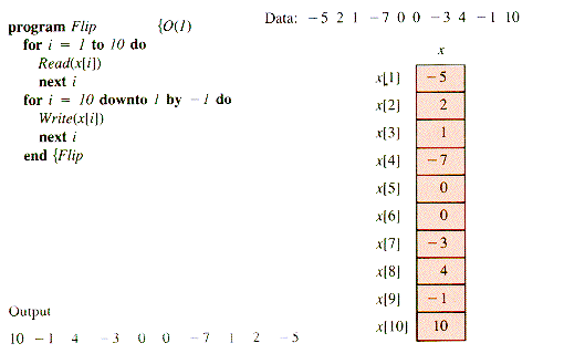
2.2 The Array as a Structure
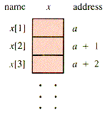
Figure 2.1
Activation
Viability
Assignment
a[i]
xRead(a[i])
Grade[3]
85.Retrieval
x
a[i]Write(a[i])
Location
2.3 Array Addresses
 , and in general, the address of a[L + i] is + i. This linear storage scheme conforms to the standard geometrical picture of an array. With it, the map from index i to its corresponding address is simply:
address
+ i - L will be treated as a variable, Alpha, so that we may discuss its computation.)procedure Main
.
.
.
err
FALSE function Map(i)address
Map(i) if i < L OR i > Uif err then ... then err
TRUE. endif
. return Alpha + i + L
. end {Mapend {MainAlpha + (-1) - (-5) = Alpha + 4
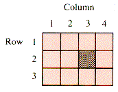
Figure 2.2
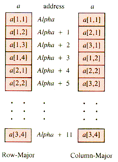
Figure 2.3
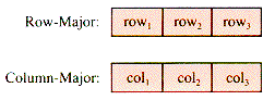
Figure 2.4
Alpha + 4 + 2 = Alpha + 4(i - 1) + (j - 1)
= Alpha + 6
Alpha + U2(i - 1) + (j - 1)
Alpha + (U2 - L2 + 1)(i - L1) + (j - L2)
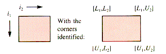
Figure 2.5
a[1,1,1],a[1,1,2], . . .,a[1,1,U3],a[1,2,1], . . .,a[1,U2U3],a[2,1,1], . . .
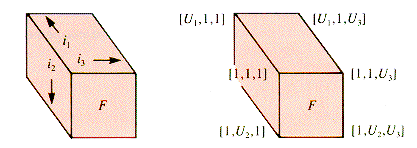
Figure 2.6
address
Alpha + (U2 -L2 + 1)(U3 - L3 + 1)(i1 - L1) +(U3 - L3 + 1)(i2 - L2) + (i3 - L3)
address = Alpha + s2
 s3 Sn(i1 - L1) + S3 Sn(i2 - L2) + + (in - Ln)
Alpha + 5 X 11 X 9(4) + 11 X 9(0) + 9(5) + 2
= Alpha + 1980 + 0 + 45 + 2
= Alpha + 2027
2.4 A Sparse and Static Table
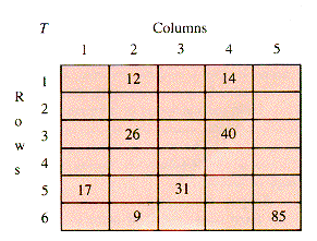
Figure 2.7
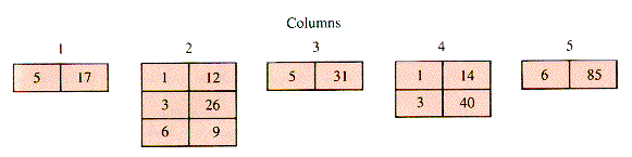
Figure 2.8
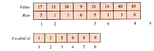
Figure 2.9
function Retrieve(i,j) {O(NI)for k
FirstInCol[j] to FirstInCol[j+1] - 1 doif Row[k] = i
then return Value[k]
endif
next k
return 0
end {RetrieveS1: Row[Dexi]
iValue[Dexi]
vDexi
Dexi + 1S2: FirstInCol[Dexj]
DexiDexj
Dexj + 1procedure CreateSST {O(NI + NC)Dexi
1Dexj
0for k
1 to NI doRead(i,j,v)
while j > Dexj do {skip empty columnsDexj
Dexj + 1FirstInCol[Dexj]
Dexiendwhile
Row[Dexi]
iValue[Dexi]
vDexi
Dexi + 1next k
while Dexj
NC do {skip empty columnsDexj
Dexj + 1FirstInCol[Dexj]
Dexiendwhile
FirstInCol[NC + 1]
NI + 1end {CreateSST2.5 Hash Tables (optional)
beef bellpepper blackpepper dillweed
onion potato olive salt
cumin carrot mushroom tomatopaste
Item HF1(Item) Item HF1(Item)
beef 18 carrot 75
onion 67 salt 52
cumin 60 blackpepper 105
dillweed 74 olive 63
bellpepper 107 tomatopaste 145
potato 87 mushroom 122
2.6 Unfolding Indices (optional)
B[1 . . 3,1 . . 3,1 . . 3],
x
y -- Retrieve[i,j,k] or Write(Retrieve[i,j,k])x
y B[i,j,k] or Write(B[i,j,k])function Retrieve(i,j,k) {O(1)Index
9 X (i -1) + 3 X (j-1) + (k-1) + 1Retrieve
Stretch[Index]end {RetrieveIndex - 1
9(i - 1) + 3(j - 1) + (k - 1)procedure Store(Value,i,j,k) {O(1)Index
9 X (i - 1) + 3 X (j - 1) + (k - 1) + 1Stretch[Index]
Valueend {StoreStore(Value,i,j,k) and Read(Value)
Store(Value,i,j,k)
B[i,j,k]
Value and Read(B[i,j,k])Summary
Further Reading
Exercises
,  , and
, and  , respectively. What are the indices for the cells with addresses + 2, + 12, + 17, + 7, + 16, + 37? if it is declared as.?
Problems
x. RetrieveBF(A,j) will check BF[j], and if A[j] has not been initialized, then it will return an error signal, otherwise it will perform RetrieveBF A[j].Origami[1 . . n1,1 . . n2]
Programs
Origami Dump
indices index
1 1 1
2 2
3 3
4 4
2 1 5
2 6
3 7
4 8
Projects