7.1 A Recursion Sampler
As others have pointed out [LEDGARD, 1981], a natural and effective definition of the word descendant is:
DEFINITION: A descendant of a person is
an offspring or
the descendant of an offspring of the person.
This definition is said to be recursive because it is in terms of itself. Two properties common to recursive definitions make it possible to search a statement to test whether or not a candidate satisfies the requirements for being recursive:
an escape clause ("an offspring") that allows a search to terminate, and
a refresh clause ("the descendant . . . ") that continues the search at a new point if escape is not invoked.
If Lottie has child Leonard has child David, then the check to test Leonard as a descendant of Lottie terminates at the first stage through the escape clause. The check for David as a descendant of Lottie must be refreshed once, continuing the search from Leonard.
Many natural-language words are defined by indirect recursion because they are defined in terms of each other. Some, like the word descendant, may be defined by direct recursion, in terms of themselves. Dictionaries are usually not so courageous.
Mathematical forms and functions can be recursive:
DEFINITION: N! = 1 for N = 0
= N X [(N - 1)!] for N > 0
DEFINITION: Xk = 1 for k = 0
= X X Xk-1 for k > 0
Both of these (and most similar examples) are closely tied to one of the pervading ideas of mathematical sciences -- Mathematical Induction, MI for short. MI is ubiquitous because it is one of the defining properties of the counting numbers 1,2,3 . . . . For the sake of completeness, here is a description of MI:
Suppose that S(n) is a statement that involves the positive integer n:
If 1. S(1) is true, and
2. S(k) is true whenever
S(1),S(2), . . . ,S(k-1) are true
then S(n) is true for all positive integers n.
The statement of MI leads naturally to iteration: prove S(1), then S(2) from it, then S(3) from S(1) and S(2) . . . .
The proof that S(n) is true for all n for some statement S has the flavor of recursion: to prove S(k), reduce it to statements about S(k - 1) and perhaps S(k - 2), . . . ,S(1) and by repetition of this, chase the truth of the supporting statements back to S(1). The chain of reasoning is then reversed for the flow of results, building back up to S(k).
A full discussion of MI is outside the scope of this book, but some of it would resemble the discussion of recursion to follow.
The simplest applications of recursion in programming are statements that act as alternates to simple iterations. For example, to find the pointer to the bottom node of a nonempty stack, pointed to by the pointer p, either an iterative or a recursive routine will do:
function ChaseTail(p) {iterative
qp
while q.Link
NIL do
qq
.Link
endwhile
return q
end {ChaseTail
function UnderDog(p) {recursive
if p.Link = NIL
then return p
else UnderDog( p.Link)
endif
end {UnderDog
UnderDog is logically valid because it repeatedly calls itself at a new point until the escape clause is invoked, and the escape clause is bound to occur. UnderDog can be implemented because a compiler that allows recursion will translate it into an iterative procedure. Very briefly, for languages in which recursion is legal, the translator of UnderDog would build a stack of pointers p, p  .Link, p
  .Link
.Link  .Link, . . . and then return the last one when the nest of invocations is unraveled. Underdog may be slower than ChaseTail, the iterated form of the operation, but both are O(n) for a stack of depth n.
Recursion can be applied at a more abstract level as it is in the English language to define data structures. For example:
DEFINITION: A linear linked list is NIL, or it is
a node linked to a linear linked list.
This definition describes a process by which a candidate may be searched for conformation, but it does not describe an algorithm. It does not force the process of refinement to terminate after a finite number of steps.
Figure 7.1 shows how the process described by the definition may be depicted.

Figure 7.1
A more specific form of the linear list definition is:
DEFINITION: A linear linked list, LinearList, is either
NIL or
a node, HeadNode, linked to a linear linked list, TaiList.
With this specification at hand, a formal structure LINLIST can be defined as any linked list that satisfies it. Given a formal data structure, there are natural operations on it, although they are not part of the definition. Examples that use a right arrow to denote "produces" are:
HEAD(LinearList)  HeadNode and TAlL(LinearList)
  TaiList, or, more abstractly:
HEAD(LinearList)  node and TAIL(LinearList)
  LinearList, where node is an item of class NODE, and LinearList is an item of class LINLIST.
These can be implemented as (rather abstract) functions:
function Head(LinearList) function Tail(LinearList)
if LinearList = NIL if LinearList = NIL
then return NIL then return NIL
else return HeadNode else return TaiList
endif endif
end {Head end {TailNeither of these functions is recursive, although the structure on which they act was defined recursively.
No part of the topic data structures is exclusively the domain of either recursion or iteration--they are both universal tools.
Problems P7.1-P7.7 are appropriate at this point.
7.1.1 From Front to Rear (optional)
7.1.1 From Front to Rear (optional)
The structure STACK of Chapter 4 was defined nonrecursively in terms of operations, yet UnderDog is a recursive operation that may be carried out on it. In fact, finding the bottom of a stack, or the last node of an instance of LINLIST, is inherently an operation requiring a repeated search. (The search may be described iteratively or recursively, but it cannot be escaped.) Essentially the same operation appears recursively in one description of the interaction between FRONT and INSERT in the structure QUEUE, as:
FRONT(INSERT(Q,i))if Empty(Q)
then i
else FRONT(Q)
endif
It is difficult to describe the relationship succinctly any other way, and the interaction between FRONT and INSERT is independent of implementation.
The trace of this interaction for a particular example demonstrates how recursion can be unraveled. After INSERT(Q, 10) is applied in Figure 7.2, then FRONT(INSERT(Q,10)) is also FRONT(Q). FRONT(Q) is FRONT (Q'), where Q' is the queue to which INSERT(Q',-5) is applied to construct Q, as in Figure 7.3.
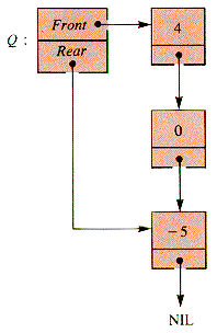
Figure 7.2
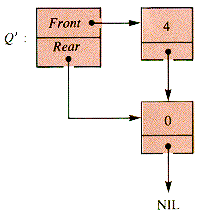
Figure 7.3
Q', in turn, is not empty, hence FRONT(Q') = FRONT(Q\"), where, as in Figure 7.4, Q' = INSERT(Q\",0).

Figure 7.4
But Q\" is not empty, and FRONT(Q\")is FRONT(INSERT(Q\"', 4)), where Q\"' is empty. The value added to an empty queue is finally the front of the queue resulting from an INSERT operation, hence:
4 = FRONT(Q\") = FRONT(Q') = FRONT(Q)
In general, FRONT(Q) is the first value not yet deleted; it can be found by tracing back through all of the insertions made since it was inserted into Q. This process of determining FRONT(Q) by applying FRONT itself as part of the process is recursive. It is a natural basis of a formal, operational definition of FRONT.
An alternate way to define a structure such as STACK, QUEUE, and LIN-LIST is to make the definition functional--expressed in terms of the operators that act on it and the relationships between them. The description of the FRONT and INSERT interaction given above serves as part of such a definition of QUEUE.
Formal definitions of the kind indicated by this section are the subject of current development and research on computer science, under the title of abstract data structures.
Any sequence may be described by a function of the positive integers. The ideal function of this kind describes a simple rule by which the nth value is to be calculated. For some sequences such as 1,2,4,9,16, . . ., a description as a function of the positive integers can be very direct: f (n) = n2.
The sequence of integers 1,1,2,3,5,8, . . . , the Fibonacci Sequence, can be taken to be f(1) = 1, f(2) = 1, f(3) = 2, f(4) = 3,f(5) = 5,f(6) = 8, . . . , but no simple description of this function is apparent. The advantage of modeling a sequence as a function is that the function may describe the sequence more succinctly than does a (partial) listing or it may provide insight into its behavior. There is such a function for the Fibonacci Sequence.
A pattern that describes the Fibonacci Sequence 1,1,2,3,5,8, . . . relates each value to the previous values: 1 + 1 = 2, 1 + 2 = 3, 2 + 3 = 5, 3 + 5 = 8, and so on. The rule that describes the nth value as a function of the previous values is:
This function may be used as a description of how to derive the nth value. For example:
This search for the nth value involves only f itself--and f invokes itself.
Self-invocation is relatively common. It appears, for example, in solving algebraic equations such as
This definition of h is in terms of itself, and the solution is h(n) = 1 - 3n, so h(1),h(2),h(3), . . . is the sequence -2,-5,-8 . . . . A major difference between h and f is in the methods of solution that can be effectively applied to them.
The solution techniques for f that are relevant here are the algorithmic ones. For example:
This is a recursive procedure because it invokes itself. It exhibits direct recursion; if, however, procedure A invokes procedure B, which itself invokes procedure A, indirect recursion is at work.
Procedure Fibol is a neat expression of the mathematical model of the Fibonacci function, but it will not work properly in a language that does not support recursion. Not all languages will support the recursive use of routines, since omitting recursion usually simplifies program compilation and speeds up the execution of programs.
If a recursive procedure is allowed in a language, then it must be possible to restructure it as an iterative procedure, or else it could not be executed on a machine that does one thing at a time. The use of recursion in programming languages can be allowed because the conversion from recursive algorithms to iterative executions is always possible and can be programmed in general into a compiler. As a direct consequence, problems having a natural expression in terms of recursion can be written that way by a programmer. The programmer can assume that the conversion to an iterative form is made correctly in translation.
The two main approaches to iterative calculations such as those needed for the Fibonacci sequence may be thought of as bottom-up iteration and top-down iteration.
Bottom-up iteration starts with known or easily found values and builds up to the desired value. A bottom-up Fibonacci calculation is:
A bottom-up Fibonacci calculation can also be done with the help of a stack in which the top values play the role of TwoBack, OneBack, and Fibo. For simplicity, assume that a particular stack is accessed by PUSH, POP, DELETE, and TOP without explicitly naming the stack. This implicit stack is similar to the stack of the FORTH machine of Part II, section F. The procedure to be developed has the flavor of the FORTH language itself, in which the standard set of stack operations is augmented with others (that can be defined in terms of the standard set). Stack operations DUP (duplicate the top value), ROT (rotate the top three values so the third comes to the top), and SUM (sum the top two values) operate as shown in Figure 7.5.
A procedure for finding f(n) with these operations is:
In order to calculate f(5) in the top-down fashion it is first necessary to calculate f(3) and f(4) upon which it depends, neither of which can be directly evaluated. In order to calculate f(4), f(3) is needed again. In one case, f(3) is "requested" by f(4), and in the other by f(5). Evaluation records can be constructed as an integer k, a value f (set to zero if not yet known), and a link back to the requesting record, shown in Figure 7.6.
Figure 7.7 pictures the calculation of f(5).
With the requests reduced to this form, the values of higher nodes can be determined from lower nodes, as shown in Figure 7.8, and finally reaching the calculation in Figure 7.9.
A direct expression of this scheme as a data structure must be deferred to Chapter 8; but, with the help of a stack, the evaluation records can be saved as they are generated and discarded as they are used. Using levels in the stack as links, f(n) can be calculated by repeating:
1. If the f-value of the top record is not zero and the level is 1, then return that value.
2. If the f-value of the top record is zero, then generate two new records (for k - 1 and k - 2) and stack them, linking them back to the record that led to their generation.
3. If the f-value is not zero for the top value but is zero for the next-to-top value, then generate two new records from the latter.
4. If the f-value is not zero for the top two values, then sum them and add the sum to the value to which they are linked. (It happens that they will be linked to the same source of their generation because records are generated in pairs.)
A trace of this process for f(5) is shown in Figure 7.10.
This picture of the stack is reflected in an array implementation of the records where array indices act as the level for both the values and the links. A new record that is linked to the record with index Level and has a given kValue may be placed on the stack by:
A record at index level can be split to produce two new records on top of the stack by:
With these operations defined, a top-down iterative calculation of the nth Fibonacci number is:
A compiler that translates the recursive function subprogram Fibol would generate activation records for each call--activation records that would resemble the evaluation records of DownStack. Note that the "n" in the definition of Fibol keeps changing with each invocation. If the records of DownStack are taken to be the actual activation records, the second stack snapshot depicts three values of n: n = 3,4, and 5 stored in k[Level] for Level = 3,2, and 1.
The availability of some language features, however, may complicate the activation records (and their generation). Even the relatively simple PL/0 compiler that generates p-code (section 4.4) must take into account the block structure of the language. Specifically, an identifier may be redefined within a subprogram, where use of the identifier has a limited scope. It is not the same variable as one named identically elsewhere. The linkage patterns within the activation stack must trace variable references back to the location of their values within the stack. That location is determined by the sequence of procedure calls during execution, in conjunction with the effects of identifier scope.
The complex problems associated with the implementation of recursive routines like Fibol can be left to language design and compiler writing. What is not to be left to them is: How can recursion be used as a design tool? When should it be used as a program design?
There is no definite answer to these questions, but--as a rule of thumb--if recursion is a natural expression of a problem solution and execution-time is not crucial, then use it.
The search through an ordered list for an arbitrary element is a common operation in computing. If output is ordered, then a search through it is efficient--the justification for sorting in the first place. The output of a program ultimately is ordered for the convenience of a search by a human or another program that accepts it as input. Sorting is justified by searching, and searching is made cost-effective by sorting.
The collection of objects to be searched in this section is essentially a file, a collection of records. The records may simply be numeric or character or string data stored in an array or list structure, or they may be more complex records. Records are assumed to contain a key, an item by which the looked-for record can be uniquely identified, and by which the file has been sorted. The sorting can be indirect through a map, but the crucial factor is whether there is independent (random) access to the key.
The problem addressed in a search, as the term is used here, is to locate an arbitrary key, Lost, somewhere in an ordered file of keys or determine that it is not there.
Two natural assumptions that can be made in casting about for efficient search techniques are (1) the file to be searched is ordered and (2) it allows independent access to keys. The simplest model of such a structure is an array containing key values that may be compared to Lost. The essential logic of the search is unchanged if the keys are not the only record values of interest or if they must be accessed through a memory map. It will be assumed here that the keys are the entries in array Key, and Lost is to be found in Key[1 . . Max].
A general (unordered) linked list, aList, with only two accessible entries (aList.Head and aList.Tail), supports only an exhaustive, linear search. (To determine that Lost is not present, every node must be checked.) The ordering of such a list structure provides for ordered output but still supports only sequential searching. The only advantage offered by ordering such a list for a linear search is that the search may be terminated as soon as the values become too large (or too small) for an absent search value to be found in the remainder of the list.
One not very efficient sequential search is LSD (for Linear Search--Dumb):
LSD has the fault that it just keeps floating along, even after finding Lost. It could be fixed in appearance by replacing Here
The for loop contains a test for the end of the search, which is what the body of the loop also contains. Only one test would suffice if it were always the case that Lost would be found. If Key is large enough, this becomes LSE (Linear Search--Extended):
This is an example of code-tuning. It can save 20-30 percent of the execution time in a long search. That is still slow, compared to the search discussed in the next section, but LSE is advantageous because it can be applied to linked lists and even unsorted lists.
A natural and recursive way to look for Lost among the values in Key[1 . . Max] stored in nondecreasing order is:
If Lost is the middle value, then quit looking. If it is smaller, then search the lower half of Key, otherwise the upper half of Key, this same way.
Each iteration of this search has roughly half as many objects to search through. If Max = 2k, then the first iteration is searching within 2k objects, the second 2k-1, and so on until there is only one value, Key[i], to compare with Lost. No more than (k + 1) = (ln Max) + 1 comparisons need to be made. In general, Max may not be a power of 2, and the search may terminate at any stage, and so a careful analysis must consider these factors. The result is of the same order, however, and the algorithmic expression of a binary search proves to be O(ln n). For large data sets this is a major difference from the O(n) needed for a linear search. (For n = 1,048,576, ln n is 20.)
Given that the essential idea of a binary search is recursive, there is still a choice between an iterative and a recursive algorithm for carrying it out. The iterative version that returns the index of the found value, or zero if it is not found, is:
It is worthwhile to trace this algorithm on a simple example.
Exercise E7.1 is appropriate at this point.
The recursive version of binary search needs to have Lower and Upper passed to it, since it operates on a segment of an array, not on an entire array. This is a fairly common effect of the change from an iterative to a recursive routine. Some local variables become parameters because they must change with each invocation of the routine. One version, initially invoked as RBS(Key,1,Max,Lost), is:
In one sense, RBS is more restrictive than IBS because it involves more parameters in the initial call. In another sense, RBS is less restrictive because it can be used to search any segment of an array, whereas IBS must search an initial segment. The latter can be easily generalized to do the same thing and both provide the same service.
More run-time overhead can be expected for RBS than for IBS because of the stacking of activation records, but both are still O(ln n) algorithms. Otherwise, for large n, RBS may use a great deal of space on the stack.
The idea of binary search is recursive, but the implementation does not have to be. The idea of dividing a data set into segments and dealing with each of them recursively has been generalized to an entire class of algorithms--the general technique is called Divide-and-Conquer (D-and-C). Among the D-and-C algorithms are sorting algorithms, one of which is the subject of section 7.5.
Exercise E7.2 is appropriate at this point.
A rich variety of stories have been formed about an apparently ancient puzzle:
There are three pegs, a, b, and c, and a stack of disks on peg a. The disks are all of different sizes and stacked so that this condition holds: no disk rests on a smaller disk. How can they be shifted to peg b (using all three pegs) so that the condition never fails on any peg during the process?
It is told that the Tibetan lamas know the solution, have been shifting 64 golden disks on three golden pegs by hand for centuries (with centuries more to go); if they succeed in some future millenium--the legend goes--the universe will end.
From the common name of the puzzle it must be known in Indochina. From its occurrence in this text, the puzzle has a role in computer science. That role is to be an example of the power of recursion.
To (legally) shift n disks from a to b, simply shift the top n - 1 disks to c, move the bottom disk from a to b, and then shift the disks on c to b. The second shift requires a change of role for the pegs, and so the information passed to the solution procedure is the number of disks to be moved, the source peg, the target peg, and the helper peg. The recursive solution is then:
If the pegs are represented by stacks, MoveOne simply pops the top value of Source, and pushes it onto Target.
Exercise E7.3, problems P7.1-P7.7, and program PG7.1 are appropriate at this point.
A number of sorting techniques involve exchanging one value (or node) for another. An obvious source of inefficiency with exchanges is that elements of a file to be sorted are exchanged more than once during the sorting process. If it were possible to exchange an element directly into its proper position (ignoring the chaos in the rest of the file at that point), then n such operations would sort the file. It would be an O(n) process.
It is not possible to make a direct exchange of an element to its correct (sorted) position because that position is not known. The correct position of an element is not even detectable without a check of the entire file for the property of being sorted. The sorted position of any element is a global property of the file.
One way to develop sorting techniques is to examine weaker properties-- those that are possessed by a sorted file but do not imply that it is necessarily sorted. A combination of such properties or the repeated establishment of one can lead to a sorted file.
Consider an array Key[1 . . Max]. If Key is sorted then for any index k, 1
Property P(k) for some k can be true with otherwise arbitrary order, and so provide a subgoal on the way to the sorting of Key. For example, Figure 7.11 has P(4), but not P(k) for other values of k, and this sequence is not sorted.
However:
If P(k) is true for every k, 1
A recursive sort called QuickSort can be developed by repeatedly establishing P(k) within the subrange Key[i] . . Key[j]. The details of QuickSort are to be found in Part II, Section O, where it is developed and implemented in Pascal.
Simply because of aesthetics some problems have become part of the repertoire of nearly everyone who is acquainted with computer science beyond an elementary programming course. Either the problem itself or its solution is elegant. One such problem is:
Place eight chess queens on a chess board so that they do not threaten each other.
A chess queen can capture another piece by moving any number of squares along one of the eight rows or eight columns or any 45-degree diagonal. Eight queens is an upper bound because no two queens can occupy the same column (or row). A solution places the nth queen in column n of the board and determines the row, Queen[n], of the nth queen so that it controls a row and diagonals distinct from those on which the other queens lie. It is possible to do this iteratively [WIRTH, 1971]. The solution presented here is recursive.
Suppose that procedure Remainder is designed so that Remainder(n) places the queens from the nth one through the eighth one to solve the problem, if possible, and also sets TruePath to TRUE if it succeeds and to FALSE otherwise. In particular, if TruePath is set TRUE by Remainder(1), the problem is solved. A solution is:
If the procedure call Remainder(n) is made with n > 8, then eight queens have been successfully placed, and it returns with TruePath = TRUE. When entered with n
The function called NextRow(i,j) simply steps through the rows i, i + 1, . . . , j and checks to see if they are safe, meaning unoccupied, with a function Safe:
Note: Cancellation is a form of backtracking--a retraction of a partially developed solution in order to try another direction. Backtracking is a general approach to solving problems often applied to binary trees and to trees, discussed in Chapters 8 and 9.
At this point in the development of EightQueens, it is no longer possible to avoid the details of how to mark and detect the presence of a queen in the rows and diagonals controlled by it.
A queen in row i, column j, also controls two diagonals, one tilting 45 degrees to the right from vertical, and one tilting 45 degrees to the left. From the view of placing another queen, it does not matter which position in a row, column, or diagonal is occupied by another queen. Rows and columns are characterized by their index. The fifteen distinct diagonals that tilt to the right are characterized by positions for which i + j is constant and has one of the values: 2,3, . . . , 16. (A move of one step up and to the right on a right-tilted diagonal decreases the row by one and increases the column by one.) Similarly, the fifteen diagonals that tilt left are characterized by i - j (in the set - 7, . . . , 7).
Figure 7.12 shows the row, column, and diagonals controlled by a queen at row 5, column 6. No information about the occupation of columns is needed since columns are possessed in sequence. Controlled rows and columns are marked in Boolean variables RowMark, TiltRight, and TiltLeft, all initialized to FALSE to indicate that they are not controlled by any queen. Documentation of an occupation is performed by setting the appropriate cells to TRUE, cancellation by resetting them to FALSE, and checking for safety by insuring that the appropriate row and diagonals are all FALSE:
Program PG7.2 and project PJ7.1 are appropriate at this point.
The records of a general list (graph) structure may contain any number of link-fields, and the links may form a tangle of great complexity. With just two link-fields a small number of nodes may form a pattern that is not any structure studied in the previous chapters--for example the pattern in Figure 7.13.
It is necessary to visit every node in such a structure to search within it, or copy it, or process the data field(s) in any way. Ways to traverse graphs based on the data structures of Chapters 8 and 9 are treated in Chapter 10. In this section, the structure is modeled by its own form.
A general record format that will serve for such a structure is:
A recursive process that visits every node of a structure and processes it is:
When Rvisit0 is applied to this example with p initially pointing to node 1, it will process nodes 1, 2, 3, 5, 6, 4, 5, 6. The multiple processing of nodes (such as 5 and 6 in this example) can cause severe problems for a user as well as inefficiency. A more serious problem is that if a link-field of node 6 pointed to node 1, it would put Rvisit0 into an infinite loop. One remedy for both problems is to introduce a Mark field set to TRUE for a node not yet processed and FALSE otherwise:
With this change, a recursive visit algorithm that processes each node only once is:
The advantage of recursive algorithms such as Rvisit is that they tend to be much simpler and more easily developed than equivalent iterative algorithms. Nevertheless, they do have shortcomings.
One problem with Rvisit itself is that if the mark-fields are all initially TRUE, then after one execution of Rvisit, they are all FALSE; and it cannot be reapplied. A separate (and similar) routine is required to complement the values of the Mark field, or Rvisit must be changed to allow p
A more severe problem with Rvisit and other recursive routines is that if a large number of nodes are involved, the run-time stack may become quite large, for it contains a copy of the information needed to continue the process for each currently unresolved link.
It is possible to derive an equivalent iterative algorithm from any recursive algorithm, but it is an awkward process and the result often benefits from rewriting. More importantly, the translation is essentially the building of explicit stacks to replace the implicit stacks that allow recursion to work.
An alternative to Rvisit that is not recursive or the explicit-stack translation of a recursive routine was discovered by Deutsch, Schorr, and Waite. A structured version, Visit, is presented in Part II, section M.
Project PJ7.2 is appropriate at this point.
A language used extensively in the field of artificial intelligence, and hence of increasing importance, is LISP. It is a working language becoming more widely available; a number of introductory books treat LISP programming. (One such is [TOURETSKY, 1983].) LISP combines a number of views about computation that give it a quality drastically different from Algol-derivations (Pascal-like languages). These include the central importance of applying functions and the use of predicates--statements with Boolean values. This section is only intended to point out how LISP is related to two themes of importance in this book: linked lists and recursion.
The central objects in a LISP program are lists, including functions that operate on them and the definitions of the functions. In the usual syntax, lists are enclosed in parentheses, and each pair of parentheses forms a list:
ITEM is not a list, but an atom.
(ITEM) is a list and has the effective structure shown in Figure 7.14
Similarly, (TWO ITEMS) has the structure shown in Figure 7.15.
The structure of ((TWO ITEMS)) is depicted in Figure 7.16.
And (((TWO ITEMS))) has the structure shown in Figure 7.17.
Storage efficiency is gained by saving atoms only once, as illustrated in Figure 7.18.
One list may be the atom of another, shown in Figure 7.19.
The recursive nature of LISP is evident in the four primitive functions below from which other functions are built. They are all designed to be used most naturally in recursive ways:
CAR returns the first atom of a list.
CDR returns the tail of a list--all but the first atom.
CONS returns a list constructed from an atom and a list.
LIST returns a list constructed from atoms.
The action of these are illustrated in Figure 7.20.
One way to retrieve an interior atom from a list is to recursively apply CDR until it is the first atom of the list, then apply CAR. That process is typical of the way LISP is written.
Note: CAR is derived from: "Contents of Address portion of Register," CDR from "Contents of Decrement portion of Register." The terms have apparently been retained for the love of the arcane found in cults.
Further pursuit of LISP itself requires a more extensive treatment than belongs in this book, but the effect of CDR, CAR, CONS, and LIST can be programmed in any language.
Project PJ7.3 is appropriate at this point.
Recursion is a fundamental way to express some relationships. When available, it can be a very convenient and delightfully succinct form for the expression of procedures.
The foundation on which language translators build recursion is a stack of activation records. Activation records are linked together on the "stack" in (possibly) interwoven lists that trace the value determinations of variables to their appropriate sources. (The p-Machine of section 4.4 and Part II, section G, is a relatively simple example of how this can be done.)
Recursion can be a marvelously easy form within which to structure an algorithm. It can also be wasteful of time and space, as illustrated by various ways to calculate the Fibonacci sequence.
The values of recursion are convenience, saving of programming time, and the development of an understanding of a problem. These may be traded for execution efficiency at the cost of the time and care required to develop an iterative solution.
Some examples in which recursion is generally deemed to be worth the runtime cost are: binary search, the Towers of Hanoi, QuickSort, and the Eight-Queens problem. (Other ways to traverse a general list are to be found in Chapter 10 and Part II, section M.)
QuickSort is frequently the sorting method of choice in applications because its average-case behavior is O(n ln n). QuickSort is an example of a recursive algorithm that tends to execute more efficiently than most iterative rivals.
The Eight-Queens solution is an example of backtracking, a programming technique of general utility.
LISP is a language that incorporates recursion and list processing into the mold of thought that it promotes in programmers.
Above all, recursion is a choice for problem solving that should be available to any programmer.
Exercises immediate applications of the text material
E7.1 Trace the procedure calls IBS(Key,6,8) and IBS(Key,6,5) when Key contains these values: Key[1] = 1, Key[2] = 3, Key[3] = 4, Key[4] = 6, Key[5] = 8, Key[6] = 10.
E7.2 Trace the calls of procedure RBS(Key, 1,6,8), RBS(Key, 1,6,5), and RBS(Key,3,6,5) with the values of Key given in E7.1.
E7.3 Trace the stacks representing the pegs in procedure Towers of section 7.4 for n = 4. (PG7. 1 asks for a program that does this.)
Problems not immediate, but requiring no major extensions of the text material
Write recursive versions of problems P7.1--P7.4:
P7.1 Search a singly linked list for a given node value.
P7.2 Search a circularly linked list for a given node value.
P7.3 Calculate N-factorial.
P7.4 Calculate the sum of the first N integers.
P7.5 (Difficult) Develop an iterative version of the Towers of Hanoi solution given in section 7.4.
P7.6 Find the GCD (Greatest Common Denominator) of two values N and M as GCD(N,M), calculated as either of them if M = N, otherwise the GCD of the smallest of them and their difference. (Use a recursive procedure.)
P7.7 Find the determinant of an N by N matrix. The determinant of A can be calculated as A[1,1] for N = 1 and the sum from j = 1 to N of (( -- 1)i+j times A[i,j] times the determinant of the ij-cofactor of A). The ij-cofactor of A is the matrix formed by deleting the ith row and the jth column of A. (Use a recursive procedure.)
Programs for trying it yourself
PG7.1 Implement procedure Towers of section 7.4 with a trace of the stacks. Run it for n = 4,5, and 6.
PG7.2 Implement the Eight-Queens solution of section 7.6 with a display routine that forms a board representation with queen markers in place.
Projects for fun and for serious students
PJ7.1 Write a program to find all solutions to the Eight-Queens puzzle.
PJ7.2 Implement Rvisit of section 7.7.
PJ7.3 Write a command-shell program to evoke functions CAR, CDR, CONS, LIST, DISPLAY, INSERT, and DELETE. The last two commands allow insertion and deletion at any depth in a list. The program is to implement DISPLAY, INSERT, and DELETE internally with the other command functions.
Comment: You may wish to implement the one-cell-per-token rule as a separate project.
7.2 The Fibonacci Connection
f(1) = 1 f(2) = 1
f(n) = f(n - 2) + f(n - 1) for n = 3,4,5, . . .
f(5) = f(3) + f(4)
= [f(1) + f(2)] + [f(2) + f(3)]
= [ 1 + 1 ] + [ 1 + [f(1) + f(2)]]
= 2 + [ 1 + [ 1 + 1 ]]
= 2 + [ 1 + 2 ]
= 2 + 3
= 5
2h(n) = h(n) - 3n + 1
function Fibo1(n) {0(2n) TRANSPARENT STACKif n = 1 then return 1 endif
if n = 2 then return 1 endif
return Fibo1(n - 2) + Fibo1(n - 1)
end {Fibo1Bottom-up Fibonacci Iteration
function UpFibo(n) {O(n)NO STACKFibo
 1
1OneBack
 1
1for i = 3 to n do
TwoBack
 OneBack
OneBack
 Fibo
FiboFibo
 TwoBack + OneBack
next i
return Fibo
end {UpFibo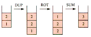
Figure 7.5
function UpStack(n) {O(n) IMPLICIT STACKPush(1)
DUP
for i = 3 to n do
DUP
ROT
SUM
next i
return Top
end {UpStackTop-down Fibonacci Iteration

Figure 7.6
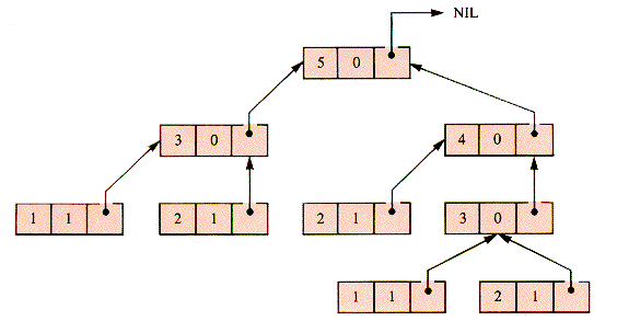
Figure 7.7
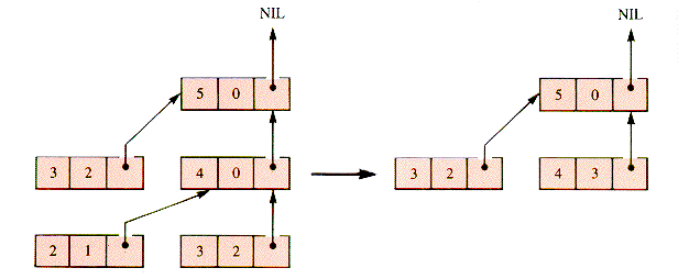
Figure 7.8
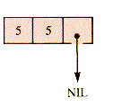
Figure 7.9

Figure 7.10
procedure NewRecord (kValue,Level)
Top
 Top + 1
if kValue < 3
then f[Top]
 1
1else f[Top]
 0
0endif
k[Top]
 kValue
Link[Top]
 Level
Levelend {NewRecordprocedure Split(Level)
kValue
 k[Level]
NewRecord(kValue-1,Level)
NewRecord(kValue-2,Level)
end {Splitfunction DownStack(n) {0(2n) EXPLICIT STACKif n
 3 then return 1 endif
Top
 0
0NewRecord(n,0)
repeat
if f[Top] = 0
then Level
 Top {split top record
Split(Level)
else if f[Top-1] = 0
then Level
 Top-1 {split next-to-top record
Split(Level)
else Level
 Link[Top] {sum top values
Sum
 f[Top] + f[Top-1]
f[Level]
 Sum
SumTop
 Top-2
Top-2endif
endif
until Top = 1
return f[1]
end {DownStack7.3 Search in an Ordered List
7.3.1 Sequential Searches
function LSD(Key,Max,Lost) {O(n)Here
 0
0for k
 1 to Max do
If Key[k] = Lost
then Here
 k
kendif
next k
return Here
end {LSD k with return k, but in some HLL languages it cannot be implemented that way.
function LSE(Key,Max,Lost) {O(n)Key[Max + 1]
 Lost
Lostk
 1
1while Key[k]
 Lost
Lostk
 k + 1
k + 1endwhile
return k
end {LSE7.3.2 Binary Searches
function IBS(Key,Max,Lost) {O(ln n) ITERATIVE BINARYLower
 1 SEARCH
Upper
 Max
Maxwhile Lower
 Upper do
Mid
 (Lower + Upper) DIV 2
case
Lost > Key[Mid]: Lower
 Mid + 1
Lost = Key[Mid]: return Mid
Lost < Key[Mid]: Upper
 Mid - 1
endcase
endwhile
return 0
end {IBSfunction RBS(Key,Lower,Upper,Lost) {O(ln n) RECURSIVE BINARYif Lower
 Upper SEARCH
then Mid
 (Lower + Upper) DIV 2
case
Lost > Key[Mid]: RBS(Key,Mid + 1, Upper,Lost)
Lost = Key[Mid]: return Mid
Lost < Key[Mid]: RBS(Key,Lower,Mid - 1,Lost)
endcase
else return 0
endif
end {RBS7.4 The Towers of Hanoi (optional)
procedure Towers(n,Source,Target,Helper)
if n = 0 then return endif
Towers(n - 1,Source,Helper,Target)
MoveOne(Source, Target)
Towers(n - 1,Helper,Target,Source)
end {Towers7.5 QuickSort (optional)
 k
k  Max, the following property holds:
Property P(k):
Key[i]
 Key[k] for 1
  i
i  k
kKey[k]
 Key[j] for k
  j
j  Max
Max
Figure 7.11
 k
k  Max, then Key is necessarily sorted.
7.6 The Eight-Queens Problem (optional)
program EightQueens
SetUp
Remainder(1)
if TruePath
then DisplayBoard
else "No solution was found."
endif
end {EightQueens 8, Remainder makes a procedure call NextRow(i,j) that searches for an available row beginning at row i. Initially NextRow is called with i = 0 and j = n and looks for the available row of lowest index, then documents the placing of queen n on that row and column n. To check the ultimate suitability of that choice, Remainder(n + 1) is called, which of course makes Remainder recursive. If it fails (TruePath = FALSE), then the row chosen by the call NextRow(i,n) is canceled (with procedure Cancel) and a row of greater index is attempted:
procedure Remainder(n)
TruePath
 FALSE
FALSEif n > 8
then TruePath
 TRUE
TRUEreturn
endif
Row
 NextRow(0,n)
while (Row
 8) AND (NOT TruePath) do
Remainder(n + 1)
if NOT TruePath
then Cancel(Row,n)
Row
 NextRow(Row,n)
endif
endwhile
end {Remainderfunction NextRow(Row,Column)
repeat
Row
 Row + 1
until Safe
if Row
 8 then Document endif
return Row
end {NextRow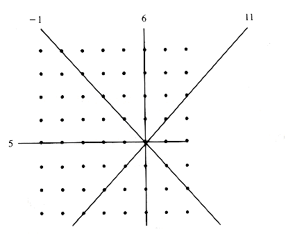
Figure 7.12
function Safe
if Row > 8
then return TRUE
else return NOT ( RowMark[Row]
OR TiltRight[Column + Row]
OR TiltLeft[Column - Row])
endif
end {Safeprocedure Document
Queen[Column]
 Row
RowRowMark[Row]
 TRUE
TRUETiltRight[Column + Row]
 TRUE
TRUETiltLeft[Column - Row]
 TRUE
TRUEend {Documentprocedure Cancel(Row,Column)
RowMark[Row]
 FALSE
FALSETiltRight[Column + Row]
 FALSE
FALSETiltLeft[Column - Row]
 FALSE
FALSEend {Cancel7.7 A General-List Visitation Algorithm (optional)

Figure 7.13
aNode = RECORD
Data: DataType
Link: ARRAY[1 .. Max] OF
 aNode
aNodeEND {aNodeprocedure Rvisit0(p) {Recursive Visit 0if p
 NIL
NILthen Process(p)
for i = 1 to Max do
Rvisit0(Link[i])
next i
endif
end {Rvisit0Node = RECORD
Data: datatype
Mark: BOOLEAN
Link: ARRAY[1 .. Max] OF
 Node
NodeEND {Nodeprocedure Rvisit(p) {Recursive Visitif (p
 NIL) AND (p
  .Mark)
then Process(p)
p
 .Mark
.Mark  FALSE
FALSEfor i = 1 to Max do
Rvisit(Link[i])
next i
endif
end {Rvisit .mark to be compared to a Boolean argument that can then be alternated between TRUE and FALSE.
7.8 LISP: Lists and Recursion (optional)
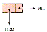
Figure 7.14

Figure 7.15
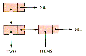
Figure 7.16

Figure 7.17

Figure 7.18
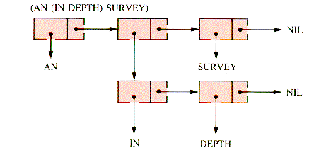
Figure 7.19
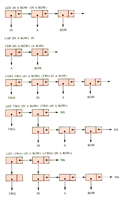
Figure 7.20
Summary
Exercises
Problems
Programs
Projects


