A positive value for a leaf node represents a winning value for the player who moves from it. A negative value represents a winning amount for the other player. Zero represents a tie.
In very few games can the board configuration be described with great brevity and the game tree drawn on a sheet of notebook paper (but see problem PW. 1). The game tree in Figure W. I is arbitrary and greatly pruned. In GT1 there are wins for Odd at nodes 5, 11, and 14 and wins for Even at nodes 6, 10, and 12.

Figure W.1
The tension in a competitive game comes from the opposition in viewpoint of the value of a configuration. Players can evaluate the node they occupy by examining the values of the children of that node. Odd wishes to maximize the payoff.
The value of node p for Odd is the maximum from the view of Odd of the values of p  . Child[i]
  for all i.
Similarly, Even wishes to minimize the payoff (to Odd), but minimizing values is equivalent to maximizing their negatives. We can combine these disparate views into a single rule:
The value of node p for the player moving from it is:
v = Maximum{ - p  .Child[i]
  .Value for all i}
With this convention, the values of the nodes of GT1 can be derived bottom-up from an assignment of values to the terminal positions represented by the leaf nodes. The value of node 2 for example is:
Maximum( - ( + 5), - ( - 10)) = + 10
The value of node 2 for Odd is - ( + 10) = -10, and so a move to node 2 would represent a loss of 10 units for Odd.
Exercise EW. 1 and problem PW. 1 are appropriate at this point.
Node evaluation as the maximum of the negative of the values (as determined by the opposition) of the children, is based on a crucial assumption:
The player in opposition always makes the move that is optimal for him or her.
The bottom-up determination of node values can be done with either recursion or with a post-order traverse--once the leaf-node values are in place, either calculated or estimated. With the assumption that leaf values are determined by a procedure Leaf Value, a recursive procedure NodeValue can be designed to assign a value v to the given node, choose the next node Choice, and return v.
function NodeValue(gt, Choice) {O(n)
ChoiceNIL
NoChildTRUE
MaxValueTooSmall {less than any possible node value
for i = 1 to MaxChild do
pgt
.Child[i]
if pNIL
then NoChildFALSE
v- NodeValue(p,Choice)
if v > MaxValue
then MaxValuev
Choicep
.Child[i]
endif
endif
next i
if NoChild
then vLeaf Value(gt)
else vMaxValue
endif
gt.Value
v
return v
end {NodeValueWhen a game tree is large, a search that reaches to the leaves of the tree is impractical, since NodeValue or its equivalent will not execute in a reasonable length of time. Most human players of games "look ahead" only a few moves to make a decision, rather than making an exhaustive search. A procedure can do the same, effectively pruning the tree.
In a look-ahead procedure, some way is needed to assign values to nodes that are not terminal and whose subtree is not traversed. Evaluation of such nodes may be done with a procedure, say BaseValue, that plays a role similar to that of Leaf Value for terminal nodes. Both procedures are highly dependent upon the game being played.
Given the existence of BaseValue, the number of nodes to be searched can be limited by restricting the depth of the search. A node being processed is some number of levels down from a root node, and an index LevelsDown can be used to track it. LevelsDown is initialized to the maximum depth to be allowed for the search and decremented at each new level. If LevelsDown = 0 at some node, then BaseValue is applied in lieu of searching the children of the node. When modified to use these tools, NodeValue can be used for a limited look-ahead determination of node values.
Problems PW.2 and PW.3 are appropriate at this point.
P>
W.1 Alpha-Beta Pruning of a Game Tree
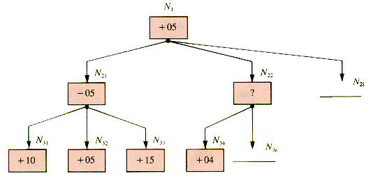
A procedure like NodeValue examines every subtree of a child, but that may not be necessary. Consider the tree fragment in Figure W.2.

Figure W.2
After (the even) node N21 has been processed, its value is known to be - 5; hence the value of N1 is at least + 5. The known minimum for a node at any point in a search of its subtrees is called its alpha value. The adversary Even controls the moves from N2j for j = 1,2, . . .; and so, as soon as N34 is found to be 4, the value of N22 is known to be at least - 4. Since the value of N22 to Even is at least - 4, it is worth no more than 4 to Odd, whence Odd will prefer N21 to N22. There is no need to traverse the other children of N22.
In general, an even node chooses its child with the smallest (odd) value and passes that value up to its (odd) parent. If an even node e has a child with a value smaller than the alpha value of its parent, then the search of the tree rooted at e may be abandoned. It is said to be pruned from the search. The children of N22 are pruned and not generated in the sense that they will not be used even if they physically exist in the structure.
The equivalent pruning on information given by the grandchildren of an even node is called beta pruning. The combination of both kinds of pruning is called alpha-beta pruning. Because of the symmetry introduced by the alternation of values in NodeValue, alpha-beta pruning is identical for odd nodes.
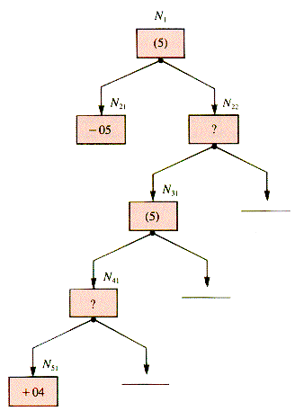
An additional phase of pruning can be initiated by passing the alpha value of a node p to a grandchild, gcp, as a lower bound, Bound. As soon as it is known that a grandchild of gcp has a value lower than Bound, the child cgcp in which it is rooted will not allow the value it passes up to gcp to be as large as Bound, and so the remaining children of cgcp can be pruned. Figure W.3 illustrates this phase.

Figure W.3
After N21 is valued, alpha(N1) is 5. This puts a lower bound of 5 on N31: as soon as N51 has a value of 4 determined for it, the children of N41 will only lower its value, and so the other children of N41 can be ignored. This form of pruning is called bounding.
Alpha-beta pruning, bounding, and level-limiting can all be incorporated into NodeValue to form:
function PruneValue(gt,Choice,Bound,Level)
if Level = 0 then return endif
ChoiceNIL
NoChildTRUE
MaxValueBound
for i = 1 to MaxChild do
pgt
.Child[i]
if pNIL
then NoChildFALSE
v- PruneChild(p, Choice, - Bound,Level - 1)
if v > MaxValue
then MaxValuev
Choicep
.Child[i]
endif
endif
next i
if NoChild
then vBound
else vMaxValue
endif
p.Value
v
return v
end {PruneValue
Exercise
Exercise immediate application of text materials
EW.1 Show how the values of the interior nodes of GT1 are derived from the values of terminal nodes.
Problems
PW.1 Draw the game tree for the game of NIM when n = 6. NIM is played by two alternating players, each of whom may pick up 1, 2, or 3 toothpicks from a pile that initially holds n. The player who empties the pile loses.
PW.2 Redesign NodeValue to be depth-limited.
PW.3 Write a search procedure that calls NodeValue.
Program for trying it yourself
PGW.1 Write a program that creates 32 random leaf-node values in the range [ - 10 . . 10], builds a game tree from them, prunes it with PruneValue, and displays the pruned tree.
Project for fun; for serious students
PJW.1 Make PGW.1 a procedure, n leaf nodes a variable, and study the mean and standard deviation of the nodes in the pruned trees as a function of n.
Problems
Program
Project


