


Dept. of Computer Science, ETH, Zurich, Switzerland
Depto. de Ciencias de la Computación, Universidad de Chile, Casilla 2777, Santiago, Chile
Centre for the New OED and Text Research, University of Waterloo, Waterloo, Ontario, Canada N2L 3G1
Abstract
We survey new indices for text, with emphasis on PAT arrays (also called suffix arrays). A PAT array is an index based on a new model of text that does not use the concept of word and does not need to know the structure of the text.
Text searching methods may be classified as lexicographical indices (indices that are sorted), clustering techniques, and indices based on hashing. In this chapter we discuss two new lexicographical indices for text, called PAT trees and PAT arrays. Our aim is to build an index for the text of size similar to or smaller than the text.
Briefly, the traditional model of text used in information retrieval is that of a set of documents. Each document is assigned a list of keywords (attributes), with optional relevance weights associated to each keyword. This model is oriented to library applications, which it serves quite well. For more general applications, it has some problems, namely:
For some indices, instead of indexing a set of keywords, all words except for those deemed to be too common (called stopwords) are indexed.
We prefer a different model. We see the text as one long string. Each position in the text corresponds to a semi-infinite string (sistring), the string that starts at that position and extends arbitrarily far to the right, or to the end of the text. It is not difficult to see that any two strings not at the same position are different. The main advantages of this model are:
This model is simpler and does not restrict the query domain. Furthermore, almost any searching structure can be used to support this view of text.
In the traditional text model, each document is considered a database record, and each keyword a value or a secondary key. Because the number of keywords is variable, common database techniques are not useful in this context. Typical data-base queries are on equality or on ranges. They seldom consider "approximate text searching."
This paper describes PAT trees and PAT arrays. PAT arrays are an efficient implementation of PAT trees, and support a query language more powerful than do traditional structures based on keywords and Boolean operations. PAT arrays were independently discovered by Gonnet (1987) and Manber and Myers (1990). Gonnet used them for the implementation of a fast text searching system, PATTM (Gonnet 1987; Fawcett 1989), used with the Oxford English Dictionary (OED). Manber and Myers' motivation was searching in large genetic databases. We will explain how to build and how to search PAT arrays.
The PAT tree is a data structure that allows very efficient searching with preprocessing. This section describes the PAT data structure, how to do some text searches and algorithms to build two of its possible implementations. This structure was originally described by Gonnet in the paper "Unstructured Data Bases" by Gonnet (1983). In 1985 it was implemented and later used in conjunction with the computerization of the Oxford English Dictionary. The name of the implementation, the PATTM system, has become well known in its own right, as a software package for very fast string searching.
In what follows, we will use a very simple model of text. Our text, or text data-base, will consist of a single (possibly very long) array of characters, numbered sequentially from one onward. Whether the text is already presented as such, or whether it can be viewed as such is not relevant. To apply our algorithms it is sufficient to be able to view the entire text as an array of characters.
A semi-infinite string is a subsequence of characters from this array, taken from a given starting point but going on as necessary to the right. In case the semi-infinite string (sistring) is used beyond the end of the actual text, special null characters will be considered to be added at its end, these characters being different than any other in the text. The name semi-infinite is taken from the analogy with geometry where we have semi-infinite lines, lines with one origin, but infinite in one direction. Sistrings are uniquely identified by the position where they start, and for a given, fixed text, this is simply given by an integer.
Example:
Sistrings can be defined formally as an abstract data type and as such present a very useful and important model of text. For the purpose of this section, the most important operation on sistrings is the lexicographical comparison of sistrings and will be the only one defined. This comparison is the one resulting from comparing two sistrings' contents (not their positions). Note that unless we are comparing a sistring to itself, the comparison of two sistrings cannot yield equal. (If the sistrings are not the same, sooner or later, by inspecting enough characters, we will have to find a character where they differ, even if we have to start comparing the fictitious null characters at the end of the text).
For example, the above sistrings will compare as follows:
22 < 11 < 2 < 8 < 1
Of the first 22 sistrings (using ASCII ordering) the lowest sistring is "a far away. . ." and the highest is "upon a time. . . ."
A PAT tree is a Patricia tree (Morrison 1968; Knuth 1973; Flajolet and Sedgewick 1986; and Gonnet 1988) constructed over all the possible sistrings of a text. A Patricia tree is a digital tree where the individual bits of the keys are used to decide on the branching. A zero bit will cause a branch to the left subtree, a one bit will cause a branch to the right subtree. Hence Patricia trees are binary digital trees. In addition, Patricia trees have in each internal node an indication of which bit of the query is to be used for branching. This may be given by an absolute bit position, or by a count of the number of bits to skip. This allows internal nodes with single descendants to be eliminated, and thus all internal nodes of the tree produce a useful branching, that is, both subtrees are non-null. Patricia trees are very similar to compact suffix trees or compact position trees (Aho et al. 1974).
Patricia trees store key values at external nodes; the internal nodes have no key information, just the skip counter and the pointers to the subtrees. The external nodes in a PAT tree are sistrings, that is, integer displacements. For a text of size n, there are n external nodes in the PAT tree and n - 1 internal nodes. This makes the tree O(n) in size, with a relatively small asymptotic constant. Later we will want to store some additional information (the size of the subtree and which is the taller subtree) with each internal node, but this information will always be of a constant size.
Figure 5.1 shows an example of a PAT tree over a sequence of bits (normally it would be over a sequence of characters), just for the purpose of making the example easier to understand. In this example, we show the Patricia tree for the text "01100100010111..." after the first 8 sistrings have been inserted. External nodes are indicated by squares, and they contain a reference to a sistring, and internal nodes are indicated by a circle and contain a displacement. In this case we have used, in each internal node, the total displacement of the bit to be inspected, rather than the skip value.
Notice that to reach the external node for the query 00101 we first inspect bit 1 (it is a zero, we go left) then bit 2 (it is zero, we go left), then bit 3 (it is a one, we go right), and then bit 5 (it is a one, we go right). Because we may skip the inspection of some bits (in this case bit 4), once we reach our desired node we have to make one final comparison with one of the sistrings stored in an external node of the current subtree, to ensure that all the skipped bits coincide. If they do not coincide, then the key is not in the tree.
So far we have assumed that every position in the text is indexed, that is, the Patricia tree has n external nodes, one for each position in the text. For some types of search this is desirable, but in some other cases not all points are necessary or even desirable to index. For example, if we are interested in word and phrase searches, then only those sistrings that are at the beginning of words (about 20% of the total for common English text) are necessary. The decision of how many sistrings to include in the tree is application dependent, and will be a trade-off between size of the index and search requirements.
In this section we will describe some of the algorithms for text searching when we have a PAT tree of our text.
Notice that every subtree of the PAT tree has all the sistrings with a given prefix, by construction. Then prefix searching in a PAT tree consists of searching the prefix in the tree up to the point where we exhaust the prefix or up to the point where we reach an external node. At this point we need to verify whether we could have skipped bits. This is done with a single comparison of any of the sistrings in the subtree (considering an external node as a subtree of size one). If this comparison is successful, then all the sistrings in the subtree (which share the common prefix) are the answer; otherwise there are no sistrings in the answer.
It is important to notice that the search ends when the prefix is exhausted or when we reach an external node and at that point all the answer is available (regardless of its size) in a single subtree. For random Patricia trees, the height is O(log n) (Pittel 1985; Apostolico and Szpankowski 1987) and consequently with PAT trees we can do arbitrary prefix searching in O(log n) time, independent of the size of the answer. In practice, the length of the query is less than O(log n), thus the searching time is proportional to the query length.
By keeping the size of each subtree in each internal node, we can trivially find the size of any matched subtree. (Knowing the size of the answer is very appealing for information retrieval purposes.) Figure 5.2 shows the search for the prefix "10100" and its answer.
We define a proximity search as finding all places where a string S1 is at most a fixed (given by the user) number of characters away from another string S2. The simplest algorithm for this type of query is to search for sl and s2. Then, sort by position the smaller of the two answers. Finally, we traverse the unsorted answer set, searching every position in the sorted set, and checking if the distance between positions (and order, if we always want s1 before s2) satisfies the proximity condition. If m1 and m2 (m1 < m2) are the respective answer set sizes, this algorithm requires (m1 + m2) log m1 time. This is not very appealing if m1 or m2 are O(n). For the latter case (when one of the strings S1 or S2 is small), better solutions based on PAT arrays have been devised by Manber and Baeza-Yates (1991).
Searching for all the strings within a certain range of values (lexicographical range) can be done equally efficiently. More precisely, range searching is defined as searching for all strings that lexicographically compare between two given strings. For example, the range "abc" . . "acc" will contain strings like "abracadabra," "acacia," "aboriginal," but not "abacus" or "acrimonious."
To do range searching on a PAT tree, we search each end of the defining intervals and then collect all the subtrees between (and including) them. It should be noticed that only O(height) subtrees will be in the answer even in the worst case (the worst case is 2 height - 1) and hence only O(log n) time is necessary in total. As before, we can return the answer and the size of the answer in time O(log n) independent of the actual size of the answer.
The longest repetition of a text is defined as the match between two different positions of a text where this match is the longest (the most number of characters) in the entire text. For a given text, the longest repetition will be given by the tallest internal node in the PAT tree, that is, the tallest internal node gives a pair of sistrings that match for the greatest number of characters. In this case, tallest means not only the shape of the tree but has to consider the skipped bits also. For a given text, the longest repetition can be found while building the tree and it is a constant, that is, will not change unless we change the tree (that is, the text).
It is also interesting and possible to search for the longest repetition not just for the entire tree/text, but for a subtree. This means searching for the longest repetition among all the strings that share a common prefix. This can be done in O(height) time by keeping one bit of information at each internal node, which will indicate on which side we have the tallest subtree. By keeping such a bit, we can find one of the longest repetitions starting with an arbitrary prefix in O(log n) time. If we want to search for all of the longest repetitions, we need two bits per internal node (to indicate equal heights as well) and the search becomes logarithmic in height and linear in the number of matches.
This type of search has great practical interest, but is slightly difficult to describe. By "most significant" or "most frequent" we mean the most frequently occurring strings within the text database. For example, finding the "most frequent" trigram is finding a sequence of three letters that appears most often within our text.
In terms of the PAT tree, and for the example of the trigrams, the number of occurrences of a trigram is given by the size of the subtree at a distance 3 characters from the root. So finding the most frequent trigram is equivalent to finding the largest subtree at a distance 3 characters from the root. This can be achieved by a simple traversal of the PAT tree which is at most O(n/average size of answer) but is usually much faster.
Searching for "most common" word is slightly more difficult but uses a similar algorithm. A word could be defined as any sequence of characters delimited by a blank space. This type of search will also require a traversal, but in this case the traversal is only done in a subtree (the subtree of all sistrings starting with a space) and does not have a constant depth; it traverses the tree to the places where each second blank appears.
We may also apply this algorithm within any arbitrary subtree. This is equivalent to finding the most frequently occurring trigram, word, and the like, that follows some given prefix.
In all cases, finding the most frequent string with a certain property requires a subtree selection and then a tree traversal which is at most O(n/k) but typically much smaller. Here, k is the average size of each group of strings of the given property. Techniques similar to alpha-beta pruning can be used to improve this search.
The main steps of the algorithm due by Baeza-Yates and Gonnet (1989) are:
a. Convert the regular expression passed as a query into a minimized deterministic finite automation (DFA), which may take exponential space/time with respect to the query size but is independent of the size of the text (Hopcroft and Ullman 1979).
b. Next eliminate outgoing transitions from final states (see justification in step (e). This may induce further minimization.
c. Convert character DFAs into binary DFAs using any suitable binary encoding of the input alphabet; each state will then have at most two outgoing transitions, one labeled 0 and one labeled 1.
d. Simulate the binary DFA on the binary digital trie from all sistrings of text using the same binary encoding as in step b. That is, associate the root of the tree with the initial state, and, for any internal node associated with state i, associate its left descendant with state j if i
e. For every node of the index associated with a final state, accept the whole subtree and halt the search in that subtree. (For this reason, we do not need outgoing transitions in final states).
f. On reaching an external node, run the remainder of the automaton on the single string determined by this external node.
For random text, it is possible to prove that for any regular expression, the average searching time is sublinear (because of step e), and of the form:
O(logm(n)n
where
The implementation of PAT trees using conventional Patricia trees is the obvious one, except for some implementation details which cannot be overlooked as they would increase the size of the index or its accessing time quite dramatically. Since this type of index is typically built over very large text databases, and the size of the index tree is linear in the size of the text, an economic implementation is mandatory.
It is easy to see that the internal nodes will be between 3 and 4 words in size. Each external node could be one word and consequently we are taking between 4n and 5n words for the index, or about 18n chars tor indexing n characters, most likely unacceptable from the practical point of view.
Second, the organization for the tree should be such that we can gain from the reading of large records external files will use physical records which are certainly larger than one internal node).
The main ideas to solve (or alleviate) both problems are
a. bucketing of external nodes, and
b. mapping the tree onto the disk using supernodes.
Collecting more than one external node is called bucketing and is an old idea in data processing. A bucket replaces any subtree with size less than a certain constant (say b) and hence saves up to b - l internal nodes. The external nodes inside a bucket do not have any structure associated with them, and any search that has to be done in the bucket has to be done on all the members of the bucket. This increases the number of comparisons for each search, in the worst case by b. On the other hand, and assuming a random distribution of keys, buckets save a significant number of internal nodes. In general, it is not possible to have all buckets full, and on average the number of keys per bucket is b In 2. Hence, instead of n - 1 internal nodes, we have about (n/bln2) internal nodes for random strings.
This means that the overhead of the internal nodes, which are the largest part of the index, can be cut down by a factor of b1n2. We have then a very simple trade-off between time (a factor of b) and space (a factor of b1n2).
Organizing the tree in super-nodes has advantages from the point of view of the number of accesses as well as in space. The main idea is simple: we allocate as much as possible of the tree in a disk page as long as we preserve a unique entry point for every page. De facto, every disk page has a single entry point, contains as much of the tree as possible, and terminates either in external nodes or in pointers to other disk pages (notice that we need to access disk pages only, as each disk page has a single entry point). The pointers in internal nodes will address either a disk page or another node inside the same page, and consequently can be substantially smaller (typically about half a word is enough). This further reduces the storage cost of internal nodes.
Unfortunately, not all disk pages will be 100 percent full. A bottom-up greedy construction guarantees at least 50 percent occupation. Actual experiments indicate an occupation close to 80 percent.
With these constraints, disk pages will contain on the order of 1,000 internal/external nodes. This means that on the average, each disk page will contain about 10 steps of a root-to-leaf path, or in other words that the total number of accesses is a tenth of the height of the tree. Since it is very easy to keep the root page of the tree in memory, this means that a typical prefix search can be accomplished with 2-3 disk accesses to read the index (about 30 to 40 tree levels) and one additional final access to verify the skipped bits (buckets may require additional reading of strings). This implementation is the most efficient in terms of disk accesses for this type of search.
The previous implementation has a parameter, the external node bucket size, b. When a search reaches a bucket, we have to scan all the external nodes in the bucket to determine which if any satisfy the search. If the bucket is too large, these costs become prohibitive.
However, if the external nodes in the bucket are kept in the same relative order as they would be in the tree, then we do not need to do a sequential search, we could do an indirect binary search (i.e., compare the sistrings referred to by the external node) to find the nodes that satisfy the search. Consequently, the cost of searching a bucket becomes 2 log b - 1 instead of b.
Although this is not significant for small buckets, it is a crucial observation that allows us to develop another implementation of PAT trees. This is simply to let the bucket grow well beyond normal bucket sizes, including the option of letting it be equal to n, that is, the whole index degenerates into a single array of external nodes ordered lexicographically by sistrings. With some additions, this idea was independently discovered by Manber and Myers (1990), who called the structures suffix arrays.
There is a straightforward argument that shows that these arrays contain most of the information we had in the Patricia tree at the cost of a factor of log2 n. The argument simply says that for any interval in the array which contains all the external nodes that would be in a subtree, in log2 n comparisons in the worst case we can divide the interval according to the next bit which is different. The sizes of the subtrees are trivially obtained from the limits of any portion of the array, so the only information that is missing is the longest-repetition bit, which is not possible to represent without an additional structure. Any operation on a Patricia tree can be simulated in O(log n) accesses. Figure 5.4 shows this structure.
It turns out that it is not neccessary to simulate the Patricia tree for prefix and range searching, and we obtain an algorithm which is O(log n) instead of O(log2 n) for these operations. Actually, prefix searching and range searching become more uniform. Both can be implemented by doing an indirect binary search over the array with the results of the comparisons being less than, equal (or included in the case of range searching), and greater than. In this way, the searching takes at most 2 log2 n - 1 comparisons and 4log2 n disk accesses (in the worst case).
The "most frequent" searching can also be improved, but its discussion becomes too technical and falls outside the scope of this section. The same can be said about "longest repetition" which requires additional supporting data structures. For regular expression searching, the time increases by a O(log n) factor. Details about proximity searching are given by Manber and Baeza-Yates (1991).
In summary, prefix searching and range searching can be done in time O(log2 n) with a storage cost that is exactly one word (a sistring pointer) per index point (sistring). This represents a significant economy in space at the cost of a modest deterioration in access time.
A historical note is worth entering at this point. Most of the research on this structure was done within the Centre for the New Oxford English Dictionary at the University of Waterloo, which was in charge of researching and implementing different aspects of the computerization of the OED from 1985. Hence, there was considerable interest in indexing the OED to provide fast searching of its 600Mb of text. A standard building of a Patricia tree in any of its forms would have required about n
Even if we were using an algorithm that used a single random access per entry point (a very minimal requirement!), the total disk time would be 119,000,000/30
Clearly we need better algorithms than the "optimal' algorithm here. We would like to acknowledge this indirect contribution by the OED, as without this real test case, we would never have realized how difficult the problem was and how much more work had to be done to solve it in a reasonable time. To conclude this note, we would say that we continue to research for better building algorithms although we can presently build the index for the OED during a weekend.
This subsection will be divided in two. First we will present the building operations, which can be done efficiently, and second, two of the most prominent algorithms for large index building.
If a portion of the text is small enough to fit in main memory together with its PAT array, then this process can be done very efficiently as it is equivalent to string sorting. Note that here we are talking about main memory; if paging is used to simulate a larger memory, the random access patterns over the text will certainly cause severe memory thrashing.
Quicksort is an appropriate algorithm for this building phase since it has an almost sequential pattern of access over the sorted file. For maximal results we can put all of the index array on external storage and apply external quicksort (see Gonnet and Baeza-Yates, section 4.4.5 [1984]) indirectly over the text. In this case it is possible to build an index for any text which together with the program can fit in main memory. With today's memory sizes, this is not a case to ignore. This is the algorithm of choice for small files and also as a building block for other algorithms.
A second case that can be solved efficiently is the case of merging two indices (to produce a single one) when the text plus twice the index of one of them fits in main memory. This algorithm is not trivial and deserves a short explanation. The text of the small file together with a PAT array for the small file (of size n1) plus an integer array of size n1 + 1 are kept in main memory. The integer array is used to count how many sistrings of the big file fall between each pair of index points in the small file (see Figure 5.5). To do this counting, the large file is read sequentially and each sistring is searched in the PAT array of the small file until it is located between a pair of points in the index. The corresponding counter is incremented. This step will require O(n2 log n1) comparisons and O(n2) characters to be read sequentially. Once the counting is finished, the merging takes place by reading the PAT array of the large file and inserting the PAT array of the small file guided by the counts (see Figure 5.6). This will require a sequential reading of n1+ n2 words. In total, this algorithm performs a linear amount of sequential input and output and O(n2 log n1) internal work, and its behavior is not only acceptable but exceptionally good.
Given these simple and efficient building blocks we can design a general index building algorithm. First we split the text file into pieces, the first piece being as large as possible to build an index in main memory. The remaining pieces are as large as possible to allow merging via the previous algorithm (small against large). Then we build indices for all these parts and merge each part.
An improvement may be made by noticing that index points at the front of the text will be merged many times into new points being added at the end. We take advantage of this by constructing partial indices on blocks of text one half the size of memory. These indices may be merged with each other, the entire merge taking place in memory. The merged index is not created at this point, since it would fill memory and could not be merged with any further index. As before, a vector of counters is kept, indicating how many entries of the first index fall between each pair of adjacent entries in the second. When the nth block of text is being indexed, the n - 1 previous indices are merged with it. The counters are accumulated with each merge. When all of the merges have been done, the counters are written to a file. When all of the blocks have been indexed and merged, the files of counters are used as instructions to merge all the partial indices.
The number of parts is O(n / m) where m is the total amount of available memory, and overall the algorithm requires O(n2 / m) sequential access and O(n2 log n / m) time. Given the sizes of present day memories and the differences of accessing time for random versus sequential access, the above quadratic algorithm would beat a linear algorithm even for databases like the Oxford English Dictionary!
An interesting property of the last version of the algorithm is that each of the merges of partial indices is independent. Therefore, all of the O((n / m)2) merges may be run in parallel on separate processors. After all merges are complete, the counters for each partial index must be accumulated and the final index merge may be done.
Another practical advantage of this algorithm is that the final index merge is done without reference to the text. Thus, at the time that the final merge is being done, the text may be removed from the system and reloaded after removal of the partial indices. In situations where the text, the final index, and the sum of partial indices may each be one or more gigabytes, this is an important consideration.
The fact that comparing sistrings through random access to disk is so expensive is a consequence of two phenomena. First, the reading itself requires some relatively slow) physical movement. Second, the amount of text actually used is a small fraction of the text made available by an I/O operation.
Here we will describe a programming technique that tries to alleviate the above problem without altering the underlying algorithms. The technique is simply to suspend execution of the program every time a random input is required, store these requests in a request pool, and when convenient/necessary satisfy all requests in the best ordering possible.
This technique works on algorithms that do not block on a particular I/O request but could continue with other branches of execution with a sufficiently high degree of parallelism. More explicitly, we have the following modules:
a. the index building program
b. a list of blocked requests
c. a list of satisfied requests
The c list is processed in a certain order. This ordering is given inversely by the likelihood of a request to generate more requests: the requests likely to generate fewer requests are processed first. Whenever the c list is exhausted or the available memory for requests is exhausted, then the b list is sorted for the best I/O performance and all the I/O is performed.
We have seen an algorithm for merging a large file against a small file, small meaning that it fits, with its index, in memory. We may also need to merge two or more large indices. We can do this by reading the text associated with each key and comparing. If we have n keys and m files, and use a heap to organize the current keys for each file being merged, this gives us O(n log m) comparisons. More importantly, it gives us n random disk accesses to fetch key values from the text. If n is 100,000,000 and we can do 50 random disk accesses per second, then this approach will take 2,000,000 seconds or about 23 days to merge the files. A second problem inherent with sistrings is that we do not know how many characters will be necessary to compare the keys. This will be addressed later.
An improvement can be made by reducing the number of random disk accesses and increasing the amount of sequential disk I/O. The sistring pointers in the PAT array are ordered lexicographically according to the text that they reference and so will be more or less randomly ordered by location in the text. Thus, processing them sequentially one at a time necessitates random access to the text. However, if we can read a sufficiently large block of pointers at one time and indirectly sort them by location in the text, then we can read a large number of keys from the text in a sequential pass. The larger the number of keys read in a sequential pass, the greater the improvement in performance. The greatest improvement is achieved when the entire memory is allocated to this key reading for each merge file in turn. The keys are then written out to temporary disk space. These keys are then merged by making a sequential pass over all the temporary files.
Thus, there are two constraints affecting this algorithm: the size of memory and the amount of temporary disk space available. They must be balanced by the relationship
memory
We must also consider how many characters are necessary for each comparison. This will be dependent on the text being indexed. In the case of the OED, the longest comparison necessary was 600 characters. Clearly it is wasteful to read (and write) 600 characters for each key being put in a temporary file. In fact, we used 48 characters as a number that allowed about 97 percent of all comparisons to be resolved, and others were flagged as unresolved in the final index and fixed in a later pass. With 48 characters per key it was possible to read 600,000 keys into a 32Mb memory. For a 600Mb text, this means that on average we are reading 1 key per kilobyte, so we can use sequential I/O. Each reading of the file needs between 30 and 45 minutes and for 120,000,000 index points it takes 200 passes, or approximately 150 hours. Thus, for building an index for the OED, this algorithm is not as effective as the large against small indexing described earlier.
However, this algorithm will work for the general case of merging indices, whether they are existing large indices for separate text files, being merged to allow simultaneous searching, or whether they are partial indices for a large text file, each constructed in memory and being merged to produce a final index. In the latter case, there are some further improvements that can be made.
Since partial indices were constructed in memory, we know that the entire text fits in memory. When we are reading keys, the entire text may be loaded into memory. Keys may then be written out to fill all available temporary disk space, without the constraint that the keys to be written must fit in memory.
Another improvement in this situation can be made by noticing that lexicographically adjacent keys will have common prefixes for some length. We can use "stemming" to reduce the data written out for each key, increasing the number of keys that can be merged in each pass.
We finish by comparing PAT arrays with two other kind of indices: signature files and inverted files.
Signature files use hashing techniques to produce an index being between 10 percent and 20 percent of the text size. The storage overhead is small; however, there are two problems. First, the search time on the index is linear, which is a drawback for large texts. Second, we may find some answers that do not match the query, and some kind of filtering must be done (time proportional to the size of the enlarged answer). Typically, false matches are not frequent, but they do occur.
On the other hand, inverted files need a storage overhead varying from 30 percent to 100 percent (depending on the data structure and the use of stopwords). The search time for word searches is logarithmic. Similar performance can be achieved by PAT arrays. The big plus of PAT arrays is their potential use in other kind of searches, that are either difficult or very inefficient over inverted files. That is the case with searching for phrases (especially those containing frequently occurring words), regular expression searching, approximate string searching, longest repetitions, most frequent searching, and so on. Moreover, the full use of this kind of index is still an open problem.
AHO, A., HOPCROFT, J., and J. ULLMAN. 1974. The Design and Analysis of Computer Algorithms. Reading, Mass.: Addison-Wesley.
APOSTOLICO, A., and W. SZPANKOWSKI. 1987. "Self-alignments in Words and their Applicatons." Technical Report CSD-TR-732, Department of Computer Science, Purdue University, West Lafayette, Ind. 47907.
BAEZA-YATES, R., and G. GONNET. 1989. "Efficient Text Searching of Regular Expressions," in ICALP'89, Lecture Notes in Computer Science 372, eds. G. Ausiello, M. DezaniCiancaglini, and S. Ronchi Della Rocca. pp. 46-62, Stresa, Italy: Springer-Verlag. Also as UW Centre for the New OED Report, OED-89-01, University of Waterloo, April, 1989.
FAWCETT, H. 1989. A Text Searching System: PAT 3.3, User's Guide. Centre for the New Oxford English Dictionary, University of Waterloo.
FLAJOLET, P. and R. SEDGEWICK. 1986. "Digital Search Trees Revisited." SIAM J Computing, 15; 748-67.
GONNET, G. 1983. "Unstructured Data Bases or Very Efficient Text Searching," in ACM PODS, vol. 2, pp. 117-24, Atlanta, Ga.
GONNET, G. 1984. Handbook of Algorithms and Data Structures. London: Addison-Wesley.
GONNET, G. 1987. "PAT 3.1: An Efficient Text Searching System. User's Manual." UW Centre for the New OED, University of Waterloo.
GONNET, G. 1988. "Efficient Searching of Text and Pictures (extended abstract)." Technical Report OED-88-02, Centre for the New OED., University of Waterloo.
HOPCROFT, J., and J. ULLMAN. 1979. Introduction to Automata Theory. Reading, Mass.: Addison-Wesley.
KNUTH, D. 1973. The Art of Computer Programming: Sorting and Searching, vol. 3. Reading, Mass.: Addison-Wesley.
MANBER, U., and R. BAEZA-YATES. 1991. "An Algorithm for String Matching with a Sequence of Don't Cares." Information Processing Letters, 37; 133-36.
MANBER, U., and G. MYERS. 1990. "Suffix Arrays: A New Method for On-line String Searches," in 1st ACM-SIAM Symposium on Discrete Algorithms, pp. 319-27, San Francisco.
MORRISON, D. 1968. "PATRICIA-Practical Algorithm to Retrieve Information Coded in Alphanumeric." JACM, 15; 514-34.
PITTEL, B. 1985. "Asymptotical Growth of a Class of Random Trees." The Annals of Probability, 13; 414-27.
5.1 INTRODUCTION
 A basic structure is assumed (documents and words). This may be reasonable for many applications, but not for others. Keywords must be extracted from the text (this is called "indexing"). This task is not trivial and error prone, whether it is done by a person, or automatically by a computer. Queries are restricted to keywords. No structure of the text is needed, although if there is one, it can be used. No keywords are used. The queries are based on prefixes of sistrings, that is, on any substring of the text.
5.2 THE PAT TREE STRUCTURE
5.2.1 Semi-infinite Strings
Text Once upon a time, in a far away land . . .
sistring 1 Once upon a time . . .
sistring 2 nce upon a time . . .
sistring 8 on a time, in a . . .
sistring 11 a time, in a far . . .
sistring 22 a far away land . . .
5.2.2 PAT Tree
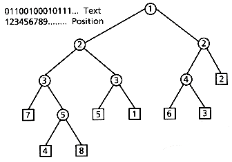
Figure 5.1: PAT tree when the sistrings 1 through 8 have been inserted
5.2.3 Indexing Points
5.3 ALGORITHMS ON THE PAT TREE
5.3.1 Prefix Searching
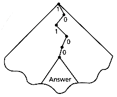
Figure 5.2: Prefix searching.
5.3.2 Proximity Searching
5.3.3 Range Searching
5.3.4 Longest Repetition Searching
5.3.5 "Most Significant" or "Most Frequent" Searching
5.3.6 Regular Expression Searching
 j for a bit 0, and associate its right descendant with state k if i k for a 1 (see Figure 5.3).
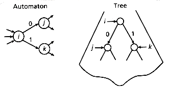
Figure 5.3: Simulating the automaton on a binary digital tree
 ) < 1, and m
 0 (integer) depend on the incidence matrix of the simulated DFA (that is, they depend on the regular expression). For details, see Baeza-Yates and Gonnet (1989).
5.4 BUILDING PAT TREES AS PATRICIA TREES
5.5 PAT TREES REPRESENTED AS ARRAYS
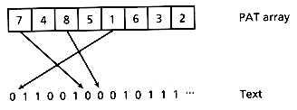
Figure 5.4: A PAT array.
5.5.1 Searching PAT Trees as Arrays
5.5.2 Building PAT Trees as Arrays
 log2(n) t hours, where n is the number of index points and t is the time for a random access to disk. As it turned out, the dictionary had about n = 119,000,000 and our computer systems would give us about 30 random accesses per second. That is, 119,000,000 27/30 60 60 = 29,750 hours or about 3.4 years. That is, we would still be building the index for the OED, 2nd ed. 60 60 24 = 45.9 days. Still not acceptable in practical terms. It is clear from these numbers that we have to investigate algorithms that do not do random access to the text, but work based on different principles.
Building PAT arrays in memory
Merging small against large PAT arrays
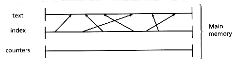
Figure 5.5: Small index in main memory
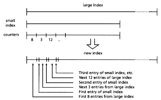
Figure 5.6: Merging the small and the large index
5.5.3 Delayed Reading Paradigm
5.5.4 Merging Large Files
number of files = temporary disk space5.6 SUMMARY
REFERENCES