


Software Productivity Consortium, Virginia Polytechnic Institute and State University
Abstract
This chapter discusses hashing, an information storage and retrieval technique useful for implementing many of the other structures in this book. The concepts underlying hashing are presented, along with two implementation strategies. The chapter also contains an extensive discussion of perfect hashing, an important optimization in information retrieval, and an O (n) algorithm to find minimal perfect hash functions for a set of keys.
Accessing information based on a key is a central operation in information retrieval. An information retrieval system must determine, given a particular value, the location (or locations) of information that have been decided to be relevant to that value. Other chapters in this book have addressed the issue; in particular, Chapters 3-6 have dealt with useful techniques for organizing files for efficient access. However, these chapters have been concerned with file-level concerns. They have not covered the fundamental underlying algorithms for organizing the indices to these files.
This chapter discusses hashing, a ubiquitous information retrieval strategy for providing efficient access to information based on a key. Under many conditions, hashing is effective both in time and space. Information can usually be accessed in constant time (although the worst-case performance can be quite poor). Space use is not optimal but is at least acceptable for most circumstances.
The material in this chapter stresses the most important concepts of hashing, and how it can be implemented. Some important theory for hashing is presented, but without derivation. Knuth (1973) provides a fuller treatment, and also gives a history and bibliography of many of the concepts in this chapter.
Hashing does have some drawbacks. As this chapter will demonstrate, they can be summarized by mentioning that it pays to know something about the data being stored; lack of such knowledge can lead to large performance fluctuations. Relevant factors include some knowledge of the domain (English prose vs. technical text, for instance), information regarding the number of keys that will be stored, and stability of data. If these factors can be predicted with some reliability--and in an information retrieval system, they usually can--then hashing can be used to advantage over most other types of retrieval algorithms.
The problem at hand is to define and implement a mapping from a domain of keys to a domain of locations. The domain of keys can be any data type--strings, integers, and so on. The domain of locations is usually the m integers between 0 and m - 1, inclusive. The mapping between these two domains should be both quick to compute and compact to represent.
Consider the problem first from the performance standpoint. The goal is to avoid collisions. A collision occurs when two or more keys map to the same location. If no keys collide, then locating the information associated with a key is simply the process of determining the key's location. Whenever a collision occurs, some extra computation is necessary to further determine a unique location for a key. Collisions therefore degrade performance.
Assume the domain of keys has N possible values. Collisions are always possible whenever N > m, that is, when the number of values exceeds the number of locations in which they can be stored. The best performance is therefore achieved by having N = m, and using a 1: 1 mapping between keys and locations. Defining such a mapping is easy. It requires only a little knowledge of the representation of the key domain. For example, if keys are consecutive integers in the range (N1, N2), then m = N2 - N1 + 1 and the mapping on a key k is k - N1. If keys are two-character strings of lowercase letters, then m = 26
Now consider compactness. If keys are drawn from the set of strings of letters up to 10 characters long--too short to be of use in information retrieval systems-- then
The problem is that the mapping is defined over all N values, that is, over all possible keys in a very large domain. In practice, no application ever stores all keys in a domain simultaneously unless the size of the domain is small. Let n be the number of keys actually stored. In most applications,
The mapping involved in hashing thus has two facets of performance: number of collisions and amount of unused storage. Optimization of one occurs at the expense of the other. The approach behind hashing is to optimize both; that is, to tune both simultaneously so as to achieve a reasonably low number of collisions together with a reasonably small amount of unused space.
The concept underlying hashing is to choose m to be approximately the maximum expected value of n. (The exact value depends on the implementation technique.) Since
The information to be retrieved is stored in a hash table. A hash table is best thought of as an array of m locations, called buckets. Each bucket is indexed by an integer between 0 and m - 1. A bucket can be empty, meaning that it corresponds to no key in use, or not empty, meaning that it does correspond to a key in use, that information has been placed in it, and that subsequent attempts to place information in it based on another key will result in a collision. (Whether "not empty" is equivalent to "full" depends on the implementation, as sections 13.4.1 and 13.4.2 show.)
The mapping between a key and a bucket is called the hash function. This is a function whose domain is that of the keys, and whose range is between 0 and m - 1, inclusive. Storing a value in a hash table involves using the hash function to compute the bucket to which a key corresponds, and placing the information in that bucket. Retrieving information requires using the hash function to compute the bucket that contains it.
For example, suppose a hash table is to be implemented with 5 buckets, and a hash function h(k) = k mod 5, where k is an integer, is used to map keys into the table. Figure 13.1 shows the hash table after the keys 1, 2, and 64 have been inserted. 1 is stored in bucket 1 because 1 mod 5 = 1, 2 is stored in bucket 2 because 2 mod 5 = 2, and so on.
This scheme works well as long as there are no collisions. The time to store and retrieve data is proportional to the time to compute the hash function. Typically, this function is very simple, and can be calculated in constant time. The space required to store the elements is that required for an array of m elements. Unless m is very large, this should not be a problem.
In practice, however, collisions should be expected. Indeed, storing more than m distinct keys into a hash table with m will always cause collisions. Even with fewer than m keys, choosing a hash function that distributes keys uniformly is sufficiently difficult that collisions can be expected to start occurring long before the hash table fills up.
This suggests two areas for further study: first, how to choose a hash function, and second, what to do when a collision occurs. Section 13.3 discusses hash functions. Section 13.4 presents two implementation techniques and the collision resolution strategies they employ. Section 13.5 explains perfect hash functions, a technique for avoiding, rather than resolving, collisions.
The choice of hash function is extremely important. The ideal function, termed a perfect hash function, would distribute all elements across the buckets such that no collisions ever occurred. As discussed in the previous section, this is desirable for performance reasons. Mapping a key to a bucket is quick, but all collision-resolution strategies take extra time--as much as
Perfect hash functions are extremely hard to achieve, however, and are generally only possible in specialized circumstances, such as when the set of elements to hash is known in advance. Another such circumstance was illustrated in Chapter 12: the bit-vector implementation of a set illustrates a perfect hash function. Every possible value has a unique bucket. This illustrates an important point: the more buckets a hash table contains, the better the performance is likely to be. Bucket quantity must be considered carefully. Even with a large number of buckets, though, a hash table is still only as good as its hash function.
The most important consideration in choosing a hash function is the type of data to be hashed. Data sets are often biased in some way, and a failure to account for this bias can ruin the effectiveness of the hash table. For example, the hash table in Figure 13.1 is storing integers that are all powers of two. If all keys are to be powers of two, then h(k) = k mod 5 is a poor choice: no key will ever map to bucket 0. As another example, suppose a hash table is be used to store last names. A 26-bucket hash table using a hash function that maps the first letter of the last name to the buckets would be a poor choice: names are much more likely to begin with certain letters than others (very few last names begin with "X").
A hash function's range must be an integer between 0 and m - 1, where m is the number of buckets. This suggests that the hash function should be of the form:
since modulo arithmetic yields a value in the desired range. Knuth (1973) suggests using as the value for m a prime number such that rk mod m = a mod m, where r is the radix of v, and a and k are small. Empirical evidence has found that this choice gives good performance in many situations. (However, Figure 13.1 shows that making m a prime number is not always desirable.)
The function f(v) should account for nuances in the data, if any are known. If v is not an integer, then the internal integer representation of its bits is used, or the first portion thereof. For example, â(v) for a nonempty charcter string might be the ASCII character-code value of the last character of the string. For a four-byte floating-point number, f(v) might be the integer value of the first byte.
Such simple-minded schemes are usually not acceptable. The problems of using the first character of a string have already been discussed; the last character is better, but not much so. In many computers, the first type of a floating-point word is the exponent, so all numbers of the same magnitude will hash to the same bucket. It is usually better to treat v as a sequence of bytes and do one of the following for f(v):
1. Sum or multiply all the bytes. Overflow can be ignored.
2. Use the last (or middle) byte instead of the first.
3. Use the square of a few of the middle bytes.
The last method, called the "mid-square" method, can be computed quickly and generally produces satisfactory results.
Once the hash function and table size have been determined, it remains to choose the scheme by which they shall be realized. All techniques use the same general approach: the hash table is implemented as an array of m buckets, numbered from 0 to m - 1. The following operations are usually provided by an implementation of hashing:
1. Initialization: indicate that the hash table contains no elements.
2. Insertion: insert information, indexed by a key k, into a hash table. If the hash table already contains k, then it cannot be inserted. (Some implementations do allow such insertion, to permit replacing existing information.)
3. Retrieval: given a key k, retrieve the information associated with it.
4. Deletion: remove the information associated with key k from a hash table, if any exists. New information indexed by k may subsequently be placed in the table.
Compare this definition with the one given in Chapter 12. There, the "information" associated with a key is simply the presence or absence of that key. This chapter considers the more general case, where other information (e.g., document names) is associated with a key.
Figure 13.2 shows a C-language interface that realizes the above operations. The routines all operate on three data types: hashTable, key, and information. The definition of the hashTable type will be left to the following sections, since particular implementation techniques require different structures. The data types of the key and the information are application-dependent; of course, the hash function must be targeted toward the key's data type.
The first implementation strategy is called chained hashing. It is so named because each bucket stores a linked list--that is, a chain--of key-information pairs, rather than a single one. The solution to a collision, then, is straightforward. If a key maps to a bucket containing no information, it is placed at the head of the list for that bucket. If a key maps to a bucket that already has information, it is placed in the list associated with that bucket. (Usually it is placed at the head of the list, on the assumption that information recently stored is likely to be accessed sooner than older information; this is also simplest to implement.) Figure 13.3 shows how the hash table from Figure 13.1 would appear if it was a chained table and all powers of two from 1 to 64 had been stored in it.
In this scheme, a bucket may have any number of elements. A hash table with m buckets may therefore store more than m keys. However, performance will degrade as the number of keys increases. Computing the bucket in which a key resides is still fast--a matter of evaluating the hash function--but locating it within that bucket (or simply determining its presence, which is necessary in all operations) requires traversing the linked list. In the worst case (where all n keys map to a single location), the average time to locate an element will be proportional to n/2. In the best case (where all chains are of equal length), the time will be proportional to n/m. It is best not to use hashing when n is expected to greatly exceed m, so n/m can be expected to remain linearly proportional to m. Usually, most chains' lengths will be close to this ratio, so the expected time is still constant.
The hashing-based implementation of Boolean operations in Chapter 12 uses chains. Most of the code from the routines Insert, Delete, Clear (for Initialize), and Member (for Retrieve) can be used directly. Chapter 12 also discussed the need for a routine to create the table. This routine had as parameters the hash function and an element-comparison routine, which shows how this information may be associated with the table.
Since the code is so similar, it will not be repeated here. Instead, a sketch is given of the differences. This is easily illustrated by considering the new data types needed. The hash table is declared as follows:
As in Chapter 12, the specifics of information and key are application-dependent, and so are not given here. The main difference from the routines in Chapter 12 lies in the need to associate the information with its key in a bucket. Hence, each bucket has a field for information. The line in Insert:
is replaced with:
The other routines differ analogously.
Sometimes, the likelihood that the number of keys will exceed the number of buckets is quite low. This might happen, for instance, when a collection of data is expected to remain static for a long period of time (as is often true in information retrieval). In such a circumstance, the keys associated with the data can be determined at the time the data is stored. As another example, sometimes the maximum number of keys is known, and the average number is expected to hover around that value. In these cases, the flexibility offered by chained hashing is wasted. A technique tailored to the amount of storage expected to be used is preferable.
This is the philosophy behind open addressing. Each bucket in the hash table can contain a single key-information pair. (That is, a bucket that is not empty is "full.") Information is stored in the table by computing the hash function value of its key. If the bucket indexed by that value is empty, the key and information are stored there. If the bucket is not empty, another bucket is (deterministically) selected. This process, called probing, repeats until an empty bucket is found.
Many strategies to select another bucket exist. The simplest is linear probing. The hash table is implemented as an array of buckets, each being a structure holding a key, associated information, and an indication of whether the bucket is empty. When a collision is detected at bucket b, bucket b + 1 is "probed" to see if it is empty. If b + 1 = m, then bucket 0 is tried. In other words, buckets are sequentially searched until an empty bucket is found.
For example, consider Figure 13.4 (a), which shows a 10-bucket hashing table containing powers of two between 1 and 16, where h(v) = v mod 10. Suppose the keys 32, 64, 128, 256, and 512 are now inserted. Key 32 collides with key 2, so it is inserted in bucket 3. Key 64 collides with key 4, so it is inserted in bucket 5. By the time key 512 is inserted, the table is as in Figure 13.4 (b), with all buckets except 0 full. Inserting key 512 necessitates the sequence of probes shown in Figure 13.4 (c). Worse, this sequence is duplicated each time 512 is retrieved. Retrieving all other elements will take little time requiring at most one extra probe, but retrieving 512 will be expensive.
This illustrates a characteristic of linear probing known as clustering: the tendency of keys to cluster around a single location. Clustering greatly increases the average time to locate keys in a hash table. It has been shown (see Sedgewick [1990], for instance) that, for a table less than two-thirds full, linear probing uses an average of less than five probes, but for tables that are nearly full, the average number of probes becomes proportional to m.
The problem is that hashing is based on the assumption that most keys won't map to the same address. Linear probing, however, avoids collisions by clustering keys around the address to which they map, ruining the suitability of nearby buckets. What is desirable is a more random redistribution. A better scheme than linear probing is to redistribute colliding keys randomly. This will not prevent collisions, but it will lessen the number of collisions due to clustering.
The redistribution can be done using some function h2(b) that, when applied to a bucket index b, yields another bucket index. In other words, the original hash function having failed, a second one is applied to the bucket. As with linear probing, another probe will be tried if the new bucket is also full. This introduces some constraints on h2. h2 = b + m would be a poor choice: it would always try the same bucket. h2 = b + m/i where m is a multiple of i would also be bad: it can only try m/i of the buckets in the table. Ideally, successive applications of h2 should examine every bucket. (Note that linear probing does this: it is simply h2(b) = (b + 1) mod m). This will happen if h2(b) = (b + i) mod m, where i is not a divisor of m. A commonly used scheme employs a formula called quadratic probing. This uses a sequence of probes of the form h + i, where i = 1, 4, 9, . . . . This is not guaranteed to probe every bucket, but the results are usually quite satisfactory.
In open addressing, it is possible to fill a hash table--that is, to place it in a state where no more information can be stored in it. As mentioned above, open addressing is best when the maximum number of keys to be stored does not exceed m. There are, however, strategies for coping when this situation arises unexpectedly. The hash table may be redefined to contain more buckets, for instance. This extension is straightforward. It can degrade performance, however, since the hash function might have been tuned to the original bucket size.
The data structures for implementing open addressing are simpler than for chained hashing, because all that is needed is an array. A suitable definition for a hash table is:
Each element of the table is a structure, not a pointer, so using a null pointer to indicate if a bucket is empty or full no longer works. Hence, a field empty has been added to each bucket. If the key is itself a pointer type, then the key field can be used to store this information. The implementation here considers the more general case.
Except for probing, the algorithms are also simpler, since no linked list manipulation is needed. Figures 13.5-13.8 show how it is done. As before, the macro:
is defined to abstract the computation of a bucket for a key.
These routines all behave similarly. They attempt to locate either an empty bucket (for Insert) or a bucket with a key of interest. This is done through some probing sequence. The basic operations of probing are initialization (setting up to begin the probe), determining if all spots have been probed, and determining the next bucket to probe. Figure 13.9 shows how quadratic probing could be implemented. The probe is considered to have failed when (m + 1)/2 buckets have been tried. In practice, this value has been shown to give good results.
Section 13.3 mentioned that the ideal hash function would avoid collisions by mapping all keys to distinct locations. This is termed a perfect hash function. A perfect hash function is ideal from a performance standpoint in that the time to locate the bucket corresponding to a particular key is always the time needed to compute the hash function. This predictability improves the ability to precisely infer performance characteristics.
Perfect hash functions are possible, but generally only when the set of keys to be hashed is known at the time the function is derived. Best of all under this condition is a minimal perfect hash function, a perfect hash function with the property that it hashes m keys to m buckets with no collisions. Not only is performance optimized, but no space is wasted in the hash table.
In general, it is difficult to find a MPHF. Knuth (1973) observes that only one in 10 million functions is a perfect hash function for mapping the 31 most frequently used English words into 41 addresses. Minimal perfect hash functions are rarer still.
This section presents an algorithm for finding minimal perfect hash functions for a given set of keys. The algorithm is not guaranteed to work, but is almost always successful. Before explaining the algorithm, it will be helpful to give some background on the topic.
One might ask whether a minimal perfect hash function (hereafter abbreviated MPHF) h exists for a set of keys. Jaeschke (1981) proves that the answer is yes. Consider the problem of mapping a set of m positive integers, bounded above by N without collisions into a hash table T with m buckets. The following algorithm defines a suitable MPHF:
The array A defines h: allowable keys map into addresses {0, ..., m - 1} and other keys map into ERROR.
This defines a MPHF, but the array A is mostly empty; since usually m
The scarcity of suitable functions suggests that it is best to search function spaces for them using computer programs. There are several strategies for doing so. The simplest is to select a class of functions that is likely to include a number of minimal perfect hash functions, and then search for a MPHF in that class by assigning different values to each of the parameters characterizing the class.
Carter and Wegman (1979) introduced the idea of a class H of functions that are universal2, that is, where no pair of distinct keys collides very often. By random selection from H, one can select candidate functions and expect that a hash function having a small number of collisions can be found quickly. This technique has been applied to dynamic hashing by Ramakrishna and Larson (1989).
Sprugnoli (1978) proposes two classes of functions, one with two and the other with four parameters, that each may yield a MPHF, but searching for usable parameter values is feasible only for very small key sets. Jaeschke (1981) suggests a reciprocal hashing scheme with three parameters, guaranteed to find a MPHF, but only practical when m
The above-mentioned "search-only" methods may (if general enough, and if enough time is allotted) directly yield a perfect hash function, with the right assignment of parameters. However, analysis of the lower bound on the size of a suitable MPHF suggests that if parameter values are not to be virtually unbounded, then there must be a moderate number of parameters to assign. In the algorithms of Cichelli (1980) and of Cercone et al. (1983) are two important concepts: using tables of values as the parameters, and using a mapping, ordering, and searching (MOS) approach (see Figure 13.10). While their tables seem too small to handle very large key sets, the MOS approach is an important contribution to the field of perfect hashing.
In the MOS approach, construction of a MPHF is accomplished in three steps. First, the mapping step transforms the key set from an original to a new universe. Second, the ordering step places the keys in a sequence that determines the order in which hash values are assigned to keys. The ordering step may partition the order into subsequences of consecutive keys. A subsequence may be thought of as a level, with the keys of each level assigned their hash values at the same time. Third, the searching step assigns hash values to the keys of each level. If the Searching step encounters a level it is unable to accommodate, it backtracks, sometimes to an earlier level, assigns new hash values to the keys of that level, and tries again to assign hash values to later levels.
Sager (1984, 1985) formalizes and extends Cichelli's approach. Like Cichelli, he assumes that a key is given as a character string. In the mapping step, three auxiliary (hash) functions are defined on the original universe of keys U:
where r is a parameter (typically
which is a triple of integers in a new universe of size mr2. The class of functions searched is
h(k) = (h0(k) + g(h1(k)) + g(h2(k)) (mod m)
where g is a function whose values are selected during the search.
Sager uses a graph that represents the constraints among keys. The mapping step goes from keys to triples to a special bipartite graph, the dependency graph, whose vertices are the h1(k) and h2(k) values and whose edges represent the words. The two vertex sets of the dependency graph are {0, . . . , r - 1} and {r, . . . , 2r - 1}. For each key k, there is an edge connecting h1(k) and h2(k), labeled by k. See Figure 13.11. Note that it is quite possible that some vertices will have no associated arcs (keys), and that some arcs may have the same pairs of vertices as their endpoints.
In the ordering step, Sager employs a heuristic called mincycle that is based on finding short cycles in the graph. Each iteration of the ordering step identifies a set of unselected edges in the dependency graph in as many small cycles as possible. The set of keys corresponding to that set of edges constitutes the next level in the ordering.
There is no proof given that a minimum perfect hash function can be found, but mincycle is very successful on sets of a few hundred keys. Mincycle takes O(m4) time and O(m3) space, while the subsequent Searching step usually takes only O(m) time.
Sager chooses values for r that are proportional to m. A typical value is r = m/2. In the case of minimal perfect hashing (m = n), it requires 2r = n computer words of lg n bits each to represent g. Fox et al. (1989a) have shown, using an argument due to Mehlhorn (1982), that a lower bound on the number of bits per key needed to represent a MPHF is approximately 1.4427. Sager's value is therefore somewhat higher than the optimal. To save space, the ratio (2r/n) must be reduced as low as possible, certainly below 1. Early work to explore and improve Sager's technique led to an implementation, with some slight improvements and with extensive instrumentation added on, described by Datta (1988). Further investigation by Fox et al. (1989a) yielded a modified algorithm requiring O(m3) time. This algorithm has been used to find MPHFs for sets of over a thousand words.
One thousand word key sets is good but still impractical for many information retrieval applications. As described in Fox et al. (1989b), Heath subsequently devised an O(m log m) algorithm, which is practical for large sets of keys. It is based on three crucial observations of previous work:
1. Randomness must be exploited whenever possible. The functions suggested by Sager do not yield distinct triples in the mapping stage with large key sets. Randomness can help improve this property.
2. The vertex degree distribution in the dependency graph is highly skewed. This can be exploited to make the ordering step much more efficient. Previously, it required up to O(m3) time; this observation reduces it to O(m log m).
3. Assigning g values to a set of related words can be viewed as trying to fit a pattern into a partially filled disk, where it is important to enter large patterns while the disk is only partially full.
Since the mapping and searching steps are O(m), the algorithm is O(m log m) with the improved ordering step.
This section presents the algorithm. It is described in terms of its three steps, plus the main program that fits these steps together. A complete implementation is too large to fit comfortably into this chapter, but it is included as an appendix.
The main program takes four parameters: the name of a file containing a list of m keys, m, a ratio for determining the size of the hash table, and the name of a file in which the output is to be written. It executes each of the three steps and, if they all succeed, creates a file containing a MPHF for the keys. Figure 13.12 outlines the main routine.
The main program is responsible for allocating enough arcs and vertices to form the dependency graph for the algorithm. "arcs" is an array of the arcs, and "vertices" an array of the vertices. Each arc corresponds to exactly one key. The data structures associated with arcs are as follows:
The arcType structure stores the ho, h1 and h2 values for an arc, plus two singly linked lists that store the vertices arcs incident to the vertices h1 and h2. The arcsType structure is an array of all arcs, with a record of how many exist.
The data structures for vertices have the form:
In vertexType, the first_edge field is the header of a linked list of arcs incident to the vertex (the next_edge values of arcType continue the list). The pred and succ fields are a doubly linked vertex list whose purpose is explained in the ordering stage. The g field ultimately stores the g function, computed during the searching stage. To save space, however, it is used for different purposes during each of the three stages.
The dependency graph created by the mapping step has 2r vertices. (The value of r is the product of m and the ratio supplied as the third parameter to the main routine. It is therefore possible to exert some control over the size of the hash function. A large value of r increases the probability of finding a MPHF at the expense of memory.) The variable vertices, of type verticesType, holds all vertices. The fields of vertices wil1 be explained as they are used in the various steps.
The code for the mapping step is shown in Figure 13.13. The step is responsible for constructing the dependency graph from the keys. This is done as follows. Three random number tables, one for each of ho, h1, h2, are initialized. The number of columns in the table determines the greatest possible key length. The number of rows is currently 128: one for each possible ASCII character. (This is not strictly necessary but helps exploit randomness.) Next, the routine map_to_triples maps each key k to a triple (ho, h1, h2) using the formulas:
That is, each function h1 is computed as the sum of the random numbers indexed by the ASCII values of the key's characters. The triple for the ith key in the input file is saved in the ith entry in the arcs array.
The mapping step then builds the dependency graph. Half of the vertices in the dependency graph correspond to the h1 values and are labeled 0, . . . , r - 1. The other half correspond to the h2 values and are labeled r, . . . , 2r - 1. There is one edge in the dependency graph for each key. A key k corresponds to an edge k, between the vertex labeled h1(k) and h2(k). There may be other edges between h1(k) and h2(k), but they are labeled with keys other than k.
Figure 13.14 shows the routine construct_graph(), which builds the dependency graph. The arcs have already been built (in map_to_triples()); what remains is to build the vertex array. Each arc is searched; the vertices associated with it are the values stored in h12[0] and h12[1]. The degree counts of these vertices are incremented, and the incidence lists associated with each vertex are updated.
Because the triples are generated using random numbers, it is possible for two triples to be identical. If this happens, a new set of random number tables must be generated, and the mapping step repeated. There is never a guarantee that all triples will be unique, although duplicates are fairly rare in practice--it can be demonstrated to be approximately r2/2m3. This value rapidly approaches 1 as m grows. To prevent infinite loops, the mapping step is never attempted more than a fixed number of times.
The goal of the ordering step is to partition the keys into a sequence of levels. The step produces an ordering of the vertices of the dependency graph (excluding those of degree 0, which do not correspond to any key). From this ordering, the partition is easily derived. If the vertex ordering is v1, . . . , vt, then the level of keys K (vi) corresponding to a vertex vi, 1
K(vi) = {kj|h1(kj) = vi, h2(kj) = vs, s < i}
Similarly, if r
K(vi) = {kj|h2(kj) = vi, h1(kj) = vs, s < i}
The rationale for this ordering comes from the observation that the vertex degree distribution is skewed toward vertices of low degree. For reasons discussed in the section on the searching step, it is desirable to have levels that are as small as possible, and to have any large levels early in the ordering.
The heuristic used to order the vertices is analogous to the algorithm by Prim (1957) for constructing a minimum spanning tree. At each iteration of Prim's algorithm, an arc is added to the minimum spanning tree that is lowest in cost such that one vertex of the arc is in the partially formed spanning tree and the other vertex is not. In the ordering step, the arc selected is the one that has maximal degree at the vertex not adjacent to any selected arcs. If several arcs are equivalent, one is chosen randomly. Since the dependency graph may consist of several disconnected graphs, the selection process will not stop after the vertices in the first component graph are ordered. Rather, it will continue to process components until all vertices of nonzero degree have been put into the ordering. Figure 13.15 shows the ordering step's implementation.
The vertex sequence is maintained in a list termed the "VS list," the head of which is the vsHead field of the vertices variable. Ordering the vertices efficiently requires quickly finding the next vertex to be added into the VS list. There are two types of vertices to consider. The first are those that start a new component graph to be explored. To handle these, the ordering step first builds (in the initialize_rList() routine) a doubly linked list of all vertices in descending order of degree. This list, whose head is in the rlistHead field of the vertices variable, and whose elements are linked via the succ and prec fields of a vertexType, can be built in linear time because of the distribution of the degrees. Since the first vertex is most likely to be within the largest component of the graph, the routine almost always correctly orders the vertices in the largest component first, rather than in the smaller components (which would produce a degraded ordering). The starting vertices tor other components are easily decided from the rList.
The second type of vertices to be added to the VS list are those adjacent to others already ordered. These are handled by keeping track of all vertices not yet ordered, but adjacent to vertices in the ordering. A heap is used to do this. The algorithm is as follows. Each component of the graph is considered in a separate iteration of the main loop of ordering: The heap is first emptied, and a vertex of maximal degree is extracted from the rList. It is marked visited (the g field is used to do so), and added to the heap.
All vertices adjacent to it are then added to the heap if they have not already been visited and are not already in the heap. Next, max_degree_vertex() removes from the heap a vertex of maximal degree with respect to others in the heap. This becomes the next "visited" vertex; it is deleted from the rList, added to the VS list, and its adjacent vertices added to the heap, as above. This process repeats until the heap is empty, at which time the next component in the graph is selected. When all components have been processed, and the heap is empty, the vertex sequence has been created.
The time to perform this step is bounded by the time to perform operations on the heap, normally O(log n). However, the skewed vertex distribution facilitates an optimization. A vertex of degree i, 1
This optimization detail is hidden by the vheap (virtual heap) module. It is not shown here but can be described quite simply. The add_to_vheap() routine takes both a vertex and its degree as parameters and can therefore determine whether to place the vertex on the heap or in a stack. The max_degree_vertex() routine obtains a vertex of maximum degree by first searching the heap; if the heap is empty, it searches stacks 5, 4, 3, 2, and 1, in that order. The implementations of these two routines are based on well-known algorithms for implementing stacks and heaps; see Sedgewick (1990), for instance.
The search step scans the VS list produced by the ordering step and tries to assign hash values to the keys, one level at a time. The hash function ultimately used has the form given in equation (1). Since h0, h1 and h2 have already been computed, what remains is to determine g.
The algorithm to compute g is again based on the insight into vertex degree distribution. The VS list contains vertices with higher degrees first; the partition into levels therefore contains larger groups of interrelated words early on. If these are processed first, the cases most likely to be troublesome are eliminated first. Note that the ordering step does not actually yield a data structure of physically distinct levels; this is simply a concept that is useful in understanding the algorithm. The levels are easily determined from the ordering in the VS list using equations (5) and (6).
The simplest way to assure that the keys are correctly fit into a hash table is to actually build a hash table. The disk variable in searching () is used for this purpose. The initialize_search() routine initializes it to an array of m slots (since the hash function is to be minimal as well as perfect), each of which is set to EMPTY. As the g function is computed for a key, the hash address h for the key is determined, and slot h in disk is marked FULL.
The implementation of the searching step is shown in Figure 13.16. Because a searching step is not guaranteed to find a suitable set of values for g, the step is repeated up to a constant number of times. Each repetition works as follows. An empty disk is allocated, all vertices are marked as not visited (in this step, the prec field holds this information), and the g field of each vertex is set to a random value. Using a random value for g often contributes to a high probability of fitting all keys.
The next vertex i in the VS list is then selected. All keys at the level of i must be fit onto the disk. This is the task of fit_pattern(), which behaves as follows. Given vertex i and disk, it examines each arc in K(vi) to see if the arc's key is at the current level (this is indicated by whether or not the vertex adjacent to i had already been visited). If so, it determines if the current values of g for vertex i and the vertices adjacent to i make any keys hash to an already-filled spot. If all keys fit, then fit-pattern() has succeeded for this level. It marks each hash address for the examined keys as FULL in disk, and terminates.
The g value determines what might be considered a "pattern." Because all keys of a particular level are associated with some vertex vi, the hash function's value for all k
This observation provides the motivation for the action to take when a collision is detected. If fit_pattern() detects a collision for some k
where s is a prime number. This means that all possible values for g can be tested in at most m tries. The searching() routine computes a table of prime numbers before computing hash addresses. It passes this table to fit-pattern(), which randomly chooses one value for the table to be used as the shift. Ideally, each vertex should have a different prime. Computing m primes is expensive, however, so a fixed number are generated. Twenty small primes have been shown, empirically, to give satisfactory results.
When the searching step is through, the main routine writes the MPHF to a file. All that is necessary is to write the size of the graph, the seed used to start random number generation, and the values of g for each vertex. Another program can then use the MPHF by:
1. Regenerating the three random number tables, which are needed to recompute h0, h1, and h2.
2. Rereading the values of g.
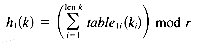
Recall that the mapping step included a call to the routine map_to_triples(), whose purpose was to compute the triples for all keys. This routine calls on compute_h012 () to actually compute the triples for a given key; compute_h012() is simply an implementation of equations (2)-(4). Given a key, then, all that is needed to compute its hash address is the code:
where tables contains the three tables, mphf the g values, and r the number of vertices on one side of the dependency graph. This is the approach used by the retrieval routine in the appendix.
The algorithm presented in this section provides a practical means to compute minimal perfect hash functions for small to extremely large sets of keys. Indeed, the algorithm has been verified on key set sizes of over one million; previous approaches could not have computed an MPHF for a set that large in reasonable time. One of its more interesting applications has been to compute the keys for an optical disk of information; see Fox (1990).
The resulting hash function is much more complex than the approaches suggested in section 13.3. Somewhat more time is necessary to use the MPHF, both to initialize it and to compute a key's value. For very small data sets, the overhead may not be justified, but for large data sets the algorithm in this section will be, on the average, much quicker. In any case, it is a constant-time algorithm, and there are always advantages to being able to predict the time needed to locate a key.
The MPHF uses a large amount of space. Ostensibly, its size is proportional to the number of vertices in the dependency graph, that is, O (r). Actually, except for very large key sets, most space is consumed by the three random number tables, which must be present at both the computation and regeneration of the MPHF. Each table has 128 rows and 150 columns, which requires over 1/4 megabyte of storage; this suggests that for small key sets, the approach suggested in section 13.5.1 might be more practical! However, an examination of the equations that access the tables (see the Mapping section step) shows that the actual number of columns used is no more than the length of the longest key. Moreover, while having 128 rows helps exploit randomness, a MPHF can be found with fewer. The implementation could therefore be rewritten to use much less space. This is left as an exercise to the reader.
CARTER, J. L., and M. N. WEGMAN. 1979. "Universal Classes of Hash Functions." J. Computer and System Sciences, 18, 143-54.
CERCONE, N., M. KRAUSE, and J. BOATES. 1983. "Minimal and Almost Minimal Perfect Hash Function Search with Application to Natural Language Lexicon Design." Computers and Mathematics with Applications 9, 215 -31.
CHANG, C . C. 1986. "Letter Oriented Reciprocal Hashing Scheme." Information Sciences 38, 243-55.
CICHELLI, R. J. 1980. "Minimal Perfect Hash Functions Made Simple." Communications of the ACM, 23, 17-19.
CORMACK, G. V., R. N. S. HORSPOOL, and M. KAISERSWERTH. 1985. "Practical Perfect Hashing." The Computer Journal 28, 54-58.
DATTA, S. 1988. "Implementation of a Perfect Hash Function Scheme." Blacksburg, Va.: Technical Report TR-89-9 (Master's Report), Department of Computer Science, Virginia Polytechnic Institute and State University.
FOX, E. A., Q. CHEN, L. HEATH, and S. DATTA. 1989a. "A More Cost Effective Algorithm for Finding Perfect Hash Functions." Paper presented at the Seventeenth Annual ACM Computer Science Conference, Louisville, KY.
FOX, E. A., Q. CHEN, and L. HEATH. 1989b. "An O (n log n) Algorithm for Finding Minimal Perfect Hash Functions." Blacksburg, Va.: TR 89-10, Department of Computer Science, Virginia Polytechnic Institute and State University.
FOX, E. A. 1990. Virginia Disc One. CD-ROM published by Virginia Polytechnic Institute and State University. Ruckersville, Va.: Nimbus Records.
JAESCHKE, G. 1981. "Reciprocal Hashing--a Method for Generating Minimal Perfect Hash Functions." Communications of the ACM, 24, 829-33.
KNUTH, D. E. 1973. The Art of Computer Programming, Vol. 3: Sorting and Searching. Reading, Mass.: Addison-Wesley.
MEHLHORN, K. 1982. "On the Program Size of Perfect and Universal Hash Functions." Paper presented at the 23rd IEEE Symposium on Foundations of Computer Science.
PRIM, R. C. 1957. "Shortest Connection Networks and Some Generalizations." Bell System Technical Journal 36.
RAMAKRISHNA, M. V., and P. LARSON. 1989. "File Organization Using Composite Perfect Hashing." ACM Transactions on Database Systems, 14, 231-63.
SAGER, T. J. 1984. "A New Method for Generating Minimal Perfect Hashing Functions." Rolla, Mo.: Technical Report CSc-84-15, Department of Computer Science, University of Missouri-Rolla.
SAGER, T. J. 1985. "A Polynomial Time Generator for Minimal Perfect Hash Functions." Communications of the ACM, 28, 523-32.
SEDGEWICK, R. 1990. Algorithms in C. Reading, Mass.: Addison-Wesley.
SPRUGNOLI, R. 1978. "Perfect Hashing Functions: a Single Probe Retrieving Method for Static Sets." Communications of the ACM, 20, 841-50.
What follows is a complete implementation of the minimal perfect hashing function algorithm. It consists of nineteen files of source code, plus a makefile (for the Unix utility make) containing compilation instructions. The beginning of each file (except the makefile, which come first) is marked by a comment consisting of a line of asterisks, with the file's name embedded in it.
13.1 INTRODUCTION
13.2 CONCEPTS OF HASHING
 26, and the mapping (using C character manipulation for ASCII) is (k [ 0 ] - ' a ' ) * (k [ 1 ] - ' a ' ) . These two mappings can be computed in constant time, and are therefore ideal from a performance standpoint.
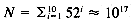 . An implementation of a mapping with m = N is impossible: no existing computer contains enough memory. The mapping that is best suited to performance is wasteful of space.
 , so only a few of the many possible keys are in use at any time. From the standpoint of compactness, the ideal representation would have m = 1; that is, all locations would be in use, no matter how many keys are in the table. All keys collide, and a strategy must exist to resolve collisions. As discussed above, any such strategy will require extra computation.
 , in theory many collisions are possible, and indeed are expected in practice. However, n is usually sufficiently small that memory consumption is not excessive; also, an attempt is made to choose a mapping that randomly spreads keys throughout the locations, lowering the probability of collision.
Figure 13.1: Visual illustration of a hash table
13.3 HASHING FUNCTIONS
 (m + n). Retrieval times become nonuniform, making performance hard to predict. A perfect hash function guarantees uniform performance.
h(v) = f(v) mod m
13.4 IMPLEMENTING HASHING
void Initialize(hashTab1e *h); /* Make h empty. */
void Insert(hashTable *h, /* Insert i into h, keyed */
key k, /* by k. */
information i);
void Delete(hashTable *h, /* Delete from h the */
key k); /* information associated */
/* with k. */
information /* Retrieve from h the */
Retrieve(hashTable *h, /* information associated */
key k); /* with k. */
#define OKAY 0 /* These values are returned */
#define DUPLICATE_KEY 1 /* by op_status(), indicating */
#define NO_SUCH_KEY 2 /* the result of the operation */
#define TABLE_FULL 3 /* last executed. */
int op_status();
Figure 13.2: Interface to a hashing implementation
13.4.1 Chained Hashing
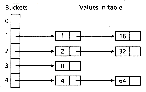
Figure 13.3: Visual illustration of a chained hash table
typedef ... information;
typedef ... key;
typedef struct be_str {key k;
information i;
struct be_str *next_datum;
};
typedef struct {int Number_Of_Buckets;
bucket_element *buckets;
int (*hashing_function)();
boolean (*comparator)();
} hashTable;
New_Element->datum = e;
New_Element->k = k;
New_Element->i = i;
13.4.2 Open Addressing
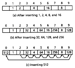
Figure 13.4: Clustering in a hash table
typedef struct {key k;
information i;
bool empty;
} bucket;
typedef struct {int number_of_buckets;
bucket *buckets;
int (*hashing_function) ();
int (*comparator) ();
} hashTable;
#define hash(h, k) ((*((h)->hashing_function))(k) % (h)->number_of_buckets)
void Initialize(h)
hashTable *h;
{register int i;
status = OKAY;
for ( i = 0; i < h->number_of_buckets; i++ )
h->buckets[i].empty = TRUE;
}
Figure 13.5: Initializing an open-addressed hash table
void Insert(h, k, i)
hashTable *h;
key k;
information i;
{register int b;
b = hash(h, k);
status = OKAY;
Initialize_Probe(h);
while ( ! h->buckets[b].empty && ! Probe_Exhausted(h) ) {if ( (*h->comparator)(k, h->buckets[b].k) ) {status = DUPLICATE_KEY;
return;
}
b = probe(h);
}
if ( h->buckets[b].empty ) {h->buckets[b].i = i;
h->buckets[b].k = k;
h->buckets[b].empty = FALSE;
}
else
status = TABLE_FULL;
}
Figure 13.6: Inserting into an open-addressed hash table
void Delete(h, k)
hashTable *h;
key k;
{register int b;
status = OKAY;
b = hash(h, k);
Initialize_Probe(h);
while ( ! h->buckets[b].empty && ! Probe_Exhausted(h) ) {if ( (*h->comparator)(k, h->buckets[b].k) ) {h->buckets[b].empty = TRUE;
return;
}
b = probe(h);
}
status = NO_SUCH_KEY;
}
Figure 13.7: Deleting from an open-addressed hash table
information Retrieve(h, k)
hashTable *h;
key k;
{register int b;
status = OKAY;
b = hash(h, k);
Initialize_Probe(h, b);
while ( ! h->buckets[b].empty && ! Probe_Exhausted(h) ) {if ( (*h->comparator)(k, h->buckets[b].k) )
return h->buckets[b].i;
b = probe(h);
}
status = NO_SUCH_KEY;
return h->buckets[0].i; /* Return a dummy value. */
}
Figure 13.8: Retrieving from an open-addressed hash table
static int number_of_probes;
static int last_bucket;
void Initialize_Probe(h, starting_bucket)
hashTable *h;
int starting_bucket;
{number_of_probes = 1;
last_bucket = starting_bucket;
}
int probe(h)
hashTable *h;
{number_of_probes++;
last_bucket = (last_bucket + number_of_probes*number_of_probes)
% h->number_of_buckets;
return last_bucket;
}
bool Probe_Exhausted(h)
hashTable *h;
{return (number_of_probes >= (h->number_of_buckets+1)/2);
}
Figure 13.9: Quadratic probing implementation
13.5 MINIMAL PERFECT HASH FUNCTIONS
13.5.1 Existence Proof
Store the keys in an array k of length m.
Allocate an array A of length N, and initialize all values to ERROR.
for ( i = 1; i < m; i++ )
A[k[i]] = i
 N, the hash function occupies too much space to be useful. In other words, efficient use of storage in hashing encompasses the representation of the hash function as well as optimal use of buckets. Both must be acceptably small if minimal perfect hashing is to be practical.
13.5.2 An Algorithm to Compute a MPHF: Concepts
 20. Chang (1986) proposes a method with only one parameter. Its value is likely to be very large, and a function is required that assigns a distinct prime to each key. However, he gives no algorithm for that function. A practical algorithm finding perfect hash functions for fairly large key sets is described by Cormack et al. (1985). They illustrate trade-offs between time and size of the hash function, but do not give tight bounds on total time to find PHFs or experimental details for very large key sets.
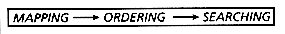
Figure 13.10: MOS method to find perfect hash functions
13.5.3 Sager's Method and Improvement
h0: U
 {0, . . . , m -- 1}
h1: U
{0, . . . , r -- 1}h2: U
{r, . . . , 2r -- 1} m/2) that determines the space to store the perfect hash function (i.e., |h| = 2r). The auxiliary functions compress each key k into a unique identifier(h0(k),h1(k),h2(k))
(1)
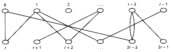
Figure 13.11: Dependency graph
13.5.4 The Algorithm
The main program
typedef struct arc { typedef struct {int h0, h12[2]; int no_arcs;
struct arc *next_edge[2]; arcType *arcArray;
} arcType; } arcsType;
main(argc, argv)
int argc;
char *argv[];
{arcsType arcs;
verticesType vertices;
int seed;
allocate_arcs( &arcs, atoi(argv[2]) );
allocate_vertices( &vertices, atoi(argv[2]) * atof(argv[3]) );
if ( mapping( arcs, vertices, &seed, argv[1] ) == NORM ) {ordering( arcs, vertices );
if ( searching ( arcs, vertices ) == NORM )
write_gfun ( vertices, seed, argv[4] );
}
}
Figure 13.12: Main program for MPHF algorithm
typedef struct { typedef struct {int g, pred, succ; int no_vertices,
struct arc *first_edge; maxDegree,
} vertexType; vsHead,
vsTail,
rlistHead;
vertexType* vertexArray;
} verticesType;
The mapping step
int mapping( key_file, arcs, vertices, seed )
char *key_file; /* in: name of file containing keys. */
arcsType *arcs; /* out: arcs in bipartite graph. */
verticesType *vertices; /* out: vertices in bipartite graph. */
int *seed; /* out: seed selected to initialize the */
/* random tables. */
{int mapping_tries = 0;
randomTablesType randomTables; /* Three random number tables. */
while ( mapping_tries++ < MAPPINGS ) {initialize_arcs( arcs );
initialize_vertices( vertices );
initialize_randomTable( randomTables, seed );
map_to_triples( key_file, arcs, vertices->no_vertices/2, randomTables );
if ( construct_graph(arcs, vertices) == NORM )
return(NORM);
}
return(ABNORM);
}
Figure 13.13: The mapping routine
int construct_graphs (arcs, vertices)
arcsType *arcs; /* in out: arcs. */
verticesType *vertices; /* in out: vertices. */
{int i, /* Iterator over all arcs. */
j, /* j = 0 and 1 for h1 and h2 side, respectively. */
status = NORM,
vertex;
for ( j = 0; j < 2; j++ ) {for ( i = 0; i < arcs->no_arcs; i++ ) {vertex = arcs->arcArray[i].h12[j]; /* Update vertex degree */
vertices->vertexArray[vertex].g++; /* count and adjacency */
arcs->arcArray[i].next_edge[j] = /* list. */
vertices->vertexArray[vertex].first_edge;
vertices->vertexArray[vertex].first_edge = &arcs ->arcArray[i];
if ( (j == 0) && check_dup( &arcs->arcArray[i] ) == ABNORM ) {status = ABNORM; /* Duplicate found. */
break;
}
/* Figure out the maximal degree of the graph. */
if ( vertices->vertexArray[vertex].g > vertices->maxDegree )
vertices->maxDegree = vertices->vertexArray[vertex].g;
}
}
return(status);
}
Figure 13.14: The construct_graph routine

(2)
(3)

(4)
The ordering step
i t is the set of edges incident to both vi and a vertex earlier in the ordering. More formally, if 0 vi < r, then(5)
vi < 2r, then(6)
void ordering( arcs, vertices )
arcsType *arcs; /* in out: the arcs. */
verticesType *vertices; /* in out: the vertices. */
{int degree, side;
vertexType *vertex;
arcType *arc;
vertices->vsHead = vertices->vsTail = NP; /* Initialize the VS list. */
initialize_rList( vertices );
allocate_vheap( arcs->no_arcs, vertices->no_vertices );
while ( vertices->rlistHead != -1 ) { /* Process each component graph. */initialize_vheap();
vertex = &vertices->vertexArray[vertices->rlistHead];
do {vertex->g = 0; /* Mark node "visited". */
delete_from_rList( vertex, vertices );
append_to_VS( vertex, vertices );
if ( vertex->first_edge != 0 ) {/* Add adjacent nodes that are not visited and */
/* not in virtual heap to the virtual heap. */
side = vertex - vertices->vertexArray >= vertices->no_vertices/2;
arc = vertex->first_edge;
while ( arc != 0 ) {int adj_node = arc->h12[(side+1)%2];
if ( (degree = vertices->vertexArray[adj_node].g) > 0 ) {add_to_vheap( &vertices->vertexArray[adj_node], degree );
vertices->vertexArray[adj_node].g *= -1;
}
arc = arc->next_edge[side];
}
}
} while ( max_degree_vertex( &vertex ) == NORM );
}
free_vheap();
}
Figure 13.15: The ordering step
i 5, is not stored on the heap. Instead, five stacks are used, stack i containing only vertices of degree i. The heap therefore contains only vertices of degree greater than 5, a small fraction of the total number. Vertices can be pushed onto and popped from a stack in constant time; the expected time of the ordering step becomes O(n) as a result.The searching step
int searching( arcs, vertices )
arcsType *arcs;
verticesType *vertices;
{int i, /* Each vertex in the VS list. */
searching_tries = 0, /* Running count of searching tries. */
status = ABNORM; /* Condition variable. */
char *disk; /* Simulated hash table. */
intSetType primes, /* Table of primes for pattern shifts. */
slotSet; /* Set of hash addresses. */
disk = (char*) owncalloc( arcs->no_arcs, sizeof(char) );
slotSet. intSetRep = (int*) owncalloc( vertices->maxDegree, sizeof(int) );
initialize_primes( arcs->no_arcs, &primes );
while ( (searching_tries++ < SEARCHINGS) && (status == ABNORM) ) {status = NORM;
i = vertices->vsHead; /* Get the highest-level vertex. */
initialize_search( arcs, vertices, disk );
while ( i != NP ) { /* Fit keys of level of vertex i onto the disk. */vertices->vertexArray[i].prec = VISIT;
if ( fit_pattern(arcs, vertices, i,
disk, &primes, &slotSet) == ABNORM ) {status = ABNORM; /* Search failed at vertex i. Try */
break; /* a new pattern. */
}
else /* Search succeeded. Proceed to next node. */
i = vertices->vertexArray[i].succ;
}
}
free( disk );
free( (char *)slotSet.intSetRep );
free( (char *)primes.intSetRep );
return(status);
}
Figure 13.16: The searching step
 K(vi) is determined in part by the value of g for vi. Any change to g will shift the hash addresses of all keys associated with a given level. K(vi), it computes a new pattern--that is, a new value for g for vertex i. All keys on the level will therefore be shifted to new addresses. The formula used to compute the new value for g is:
g
 ( g + s) mod m
Using the MPHF
arcType arc;
compute_h012 ( no_arcs, r, tables, key, &arc );
hash = abs (arc.h0 +
mphf->gArray[arc.h12[0]] +
mphf->gArray[arc. h12[1]]
) % mphf->no_arcs;
Discussion
REFERENCES
APPENDIX: MPHF IMPLEMENTATION
#
# Makefile for the minimal perfect hash algorithm.
#
# Directives:
# phf Make phf, a program to generate a MPHF.
#
# regen_mphf.a Make an object code library capable of
# regenerating an MPHF from the specification
# file generated by phf.
#
# regen_driver Make regen_driver, a program to test
# the code in regen_mphf.a
#
# all (default) Make the three above items.
#
# regression Execute a regression test. The phf program
# should terminate indicating success. The
# regen_driver program silently checks its
# results; no news is good news.
#
# lint Various flavors of consistency checking.
# lint_phf
# lint_regen
#
#
COMMON_OBJS= compute_hfns.o randomTables.o pmrandom.o support.o
COMMON_SRCS= compute_hfns.c randomTables.c pmrandom.c support.c
COMMON_HDRS= compute_hfns.h randomTables.h pmrandom.h support.h \
const.h types.h
MPHF_OBJS= main.o mapping.o ordering.o searching.o vheap.o
MPHF_SRCS= main.c mapping.c ordering.c searching.c vheap.c
MPHF_HDRS= vheap.h
REGEN_OBJS= regen_mphf.o
REGEN_SRCS= regen_mphf.c
REGEN_HDRS= regen_mphf.h
RD_OBJS= regen_driver.o
RD_SRCS= regen_driver.c
PHFLIB= regen_mphf.a
CFLAGS= -O
LDFLAGS=
LIBS= -lm
all: phf regen_driver
phf: $(PHFLIB) $(MPHF_OBJS)
$(CC) -o phf $ (LDFLAGS) $ (MPHF_OBJS) $ (PHFLIB) -lm
$(PHFLIB): $(REGEN_OBJS) $ (COMMON_OBJS)
ar r $ (PHFLIB) $?
ranlib $ (PHFLIB)
regen_driver: $(RD_OBJS) $ (PHFLIB)
$(CC) $ (LDFLAGS) -o regen_driver $(RD_OBJS) $(PHFLIB) $(LIBS)
regression: phf regen_driver
. /phf keywords 'wc -l < keywords' 0.8 /tmp/hashing-output
. /regen_driver /tmp/hashing-output keywords > /tmp/hashed-words
rm /tmp/hashing-output /tmp/hashed-words
lint: lint_phf lint_regen
lint_phf:
lint $(MPHF_SRCS) $(COMMON_SRCS) $(LIBS)
lint_regen:
lint $(RD_SRCS) $(REGEN_SRCS) $(COMMON_SRCS) $(LIBS)
compute_hfns.o: const.h randomTables.h types.h
main.o: const.h types.h support.h
mapping.o: const.h pmrandom.h compute_hfns.h types.h support.h
ordering.o: const.h types.h vheap.h support.h
randomTables.o: const.h pmrandom.h randomTables.h types.h
searching.o: const.h pmrandom.h support.h types.h
support.o: const.h types.h support.h
pmrandom.o: pmrandom.h
vheap.o: const.h support.h types.h vheap.h
/*************************** compute_hfns.h ***************************
Purpose: External declarations for computing the three h functions
associated with a key.
Provenance: Written and tested by Q. Chen and E. Fox, March 1991.
Edited and tested by S. Wartik, April 1991.
Notes: None.
**/
#ifdef __STDC__
extern void compute_h012( int n, int r, randomTablesType tables,
char *key, arcType *arc );
#else
extern void compute_h012();
#endif
/****************************** const.h *******************************
Purpose: Define globally-useful constant values.
Provenance: Written and tested by Q. Chen and E. Fox, March 1991.
Edited and tested by S. Wartik, April 1991.
Notes: None.
**/
#define MAX_INT ((unsigned)(~0)) >> 1 /* Maximum integer. */
#define NP -1 /* Null pointer for array-based linked lists. */
#define NORM 0 /* Normal return. */
#define ABNORM -1 /* Abnormal return. */
#define MAPPINGS 4 /* Total number of mapping runs */
#define SEARCHINGS 10 /* Total number of searching runs. */
#define MAX_KEY_LENG COLUMNS /* Maximum length of a key. */
#define PRIMES 20 /* Number of primes, used in searching stage. */
#define NOTVISIT 0 /* Indication of an un-visited node. */
#define VISIT 1 /* Indication of a visited node. */
#define EMPTY '0' /* Indication of an empty slot in the disk. */
#define FULL '1' /* Indication of a filled slot in the disk. */
/***************************** pmrandom.h *****************************
Purpose: External declarations for random-number generator
package used by this program.
Provenance: Written and tested by Q. Chen and E. Fox, March 1991.
Edited by S. Wartik, April 1991.
Notes: The implementation is better than the random number
generator from the C library. It is taken from Park and
Miller's paper, "Random Number Generators: Good Ones are
Hard to Find," in CACM 31 (1988), pp. 1192-1201.
**/
#ifdef __STDC__
extern void setseed(int); /* Set the seed to a specified value. */
extern int pmrandom(); /* Get next random number in the sequence. */
extern int getseed(); /* Get the current value of the seed. */
#else
extern void setseed();
extern int pmrandom();
extern int getseed();
#endif
#define DEFAULT_SEED 23
/************************** randomTables.h ****************************
Purpose: External definitions for the three random number tables.
Provenance: Written and tested by Q. Chen and E. Fox, March 1991.
Edited and tested by S. Wartik, April 1991.
**/
#define NO_TABLES 3 /* Number of random number tables. */
#define ROWS 128 /* Rows of the random table (suitable for char). */
#define COLUMNS 150 /* Columns of the random table. */
typedef int randomTablesType[NO_TABLES] [ROWS] [COLUMNS]; /* random number table */
#ifdef __STDC__
extern void initialize_randomTable( randomTablesType tables, int *seed );
#else
extern void initialize_randomTable();
#endif
/**************************** regen_mphf.h *****************************
Purpose: External declarations for regenerating and using
an already-computed minimal perfect hashing function.
Provenance: Written and tested by Q. Chen and E. Fox, March 1991.
Edited and tested by S. Wartik, April 1991.
Notes: None.
**/
typedef struct {int no_arcs; /* Number of keys (arcs) in the key set. */
int no_vertices; /* Number of vertices used to compute MPHF. */
int seed; /* The seed used for the random number tables. */
randomTablesType tables; /* The random number tables. */
int *gArray; /* The array to hold g values. */
} mphfType;
#ifdef __STDC__
extern int regen_mphf ( mphfType *mphf, char *spec_file );
extern void release_mphf ( mphfType *mphf );
extern int retrieve ( mphfType *mphf, char *key );
#else
extern int regen_mphf ();
extern void release_mphf ();
extern int retrieve ();
#endif
/***************************** support.h ******************************
Purpose: External interface for support routines.
Provenance: Written and tested by Q. Chen and E. Fox, March 1991.
Edited and tested by S. Wartik, April 1991.
Notes: None.
**/
#ifdef __STDC__
extern char *owncalloc(int n, int size);
extern char *ownrealloc(char *area, int new_size);
extern void write_gfun(arcsType *arcs, verticesType *vertices,
int tbl_seed, char *spec_file);
extern int verify_mphf(arcsType *arcs, verticesType *vertices);
#else
extern char *owncalloc();
extern char *ownrealloc();
extern void write_gfun();
extern int verify_mphf();
#endif
/****************************** types.h *******************************
Purpose: Define globally-useful data types.
Provenance: Written and tested by Q. Chen and E. Fox, March 1991.
Edited and tested by S. Wartik, April 1991.
Notes: None.
**/
#include "const.h"
typedef struct arc { /* arc data structure */int h0, /* h0 value */
h12[2]; /* h1 and h2 values */
struct arc *next_edge[2]; /* pointer to arc sharing same h1 or */
} arcType; /* h2 values */
typedef struct { /* vertex data structure */struct arc *first_edge; /* pointer to the first adjacent edge */
int g, /* g value. */
prec, /* backward pointer of the vertex-list */
succ; /* forward pointer of the vertex-list */
} vertexType;
typedef struct { /* arcs data structure */int no_arcs; /* number of arcs in the graph */
arcType*arcArray; /* arc array */
} arcsType;
typedef struct { /* vertices data structure */int no_vertices, /* number of vertices in the graph */
maxDegree, /* max degree of the graph */
vsHead, /* VS list head */
vsTail, /* VS list tail */
rlistHead; /* remaining vertex list head */
vertexType* vertexArray; /* vertex array */
} verticesType;
typedef struct { /* integer set data structure */int count, /* number of elements in the set */
*intSetRep; /* set representation */
} intSetType;
/****************************** vheap.h *******************************
Purpose: Define a "virtual heap" module.
Provenance: Written and tested by Q. Chen and E. Fox, March l99l.
Edited and tested by S. Wartik, April l99l.
Notes: This isn't intended as a general-purpose stack/heap
implementation. It's tailored toward stacks and heaps
of vertices and their degrees, using a representation suitable
for accessing them (in this case, an integer index into
the vertices->verex array identifies the vertex).
**/
#ifdef _STDC_
extern void allocate_vheap( int no_arcs, int no_vertices );
extern void initialize_vheap();
extern void add_to_vheap ( vertexType *vertex, int degree );
extern int max_degree_vertex ( vertexType **vertex );
extern void free_vheap();
#else
extern void allocate_vheap();
extern void initialize_vheap();
extern void add_to_vheap ();
extern int max_degree_vertex ();
extern void free_vheap();
#endif
/***************************** compute_hfns.c *****************************
Purpose: Computation of the three h functions associated with
a key.
Provenance: Written and tested by Q. Chen and E. Fox, March l99l.
Edited and tested by S. Wartik, April l99l.
Notes: None.
**/
#include <stdio.h>
#include <string.h>
#include "types.h"
#include "randomTables.h"
/*************************************************************************
compute_h012( int, int, randomTablesType, char*, arcType* )
Return: void
Purpose: Compute the triple for a key. On return, the h0 and h12
fields of "arc" have the triple's values.
**/
void compute_h012(n, r, tables, key, arc)
int n, /* in: number of arcs. */
r; /* in: size of h1 or h2 side of the graph. */
randomTablesType tables; /* in: pointer to the random tables. */
char *key; /* in: key string. */
arcType *arc; /* out: the key's arc entry. */
{int i, /* Iterator over each table. */
j, /* Iterator over each character in "key". */
sum[NO_TABLES], /* Running sum of h0, h1 and h2 values. */
length; /* The length of "key". */
length = strlen(key) ;
sum[0] = sum[1] = sum[2] = 0 ;
for ( i = 0; i < NO_TABLES; i++ ) /* Sum over all the characters */
for ( j = 0; j < length; j++ ) /* in the key. */
sum[i] += table[i][(key[j]%ROWS)][j];
arc->h0 = abs( sum[0] ) % n; /* Assign mappings for each */
arc->h12[0] = abs( sum[1] ) % r; /* of h0, h1, and h2 according */
arc->hl2[1] = abs( sum[2] ) % r + r; /* to the sums computed. */
}
/******************************** main.c *********************************
Purpose: Main routine, driving the MPHF creation.
Provenance: Written and tested by Q. Chen and E. Fox, March 1991.
Edited and tested by S. Wartik, April 1991.
Notes: When compiled, the resulting program is used as follows:
phf I L R O
where:
I Name of the file to be used as input. It should contain
one or more newline-terminated strings.
L The number of lines in I.
R A real number, giving a ratio between L and the size of
the hashing function generated. 1.0 is usually a viable
value. In general, L*R should be an integer.
O Name of a file to be used as output. It will contain
the MPHF if one is found.
**/
#include <stdio.h>
#include <math.h>
#include <string.h>
#include "types.h"
#include "support.h"
#ifdef __STDC__
extern void ordering( arcsType *arcs, verticesType *vertices );
extern void allocate_arcs( arcsType* arcs, int n );
extern void allocate_vertices( verticesType* vertices, int n );
extern void free_arcs( arcsType* arcs );
extern void free_vertices( verticesType* vertices );
extern void exit();
#else
extern void ordering();
extern void allocate_arcs();
extern void allocate_vertices();
extern void free_arcs();
extern void free_vertices();
extern void exit();
#endif
/*************************************************************************
main(argc, argv)
Returns: int -- zero on success, non-zero on failure.
Purpose: Take the inputs and call three routines to carry out mapping,
ordering and searching three tasks. If they all succeed,
write the MPHF to the spec file.
**/
main( argc, argv )
int argc;
char *argv[ ]; /* arg1: key file; arg2: key set size; */
/* arg3: ratio; arg4: spec file */
{int status, /* Return status variable. */
seed; /* Seed used to initialize the three random */
/* tables. */
char *key_file_name,
*specification_file_name;
int lines_in_keyword_file;
double ratio;
arcsType arcs; /* These variables hold all the arcs */
verticesType vertices; /* and vertices generated. */
if ( argc != 5 ) {fprintf(stderr, "Usage: %s keywords kw-lines ratio output-file\n",
argv[0]);
exit(1);
}
key_file_name = argv[1];
if ( (lines_in_keyword_file = atoi(argv[2])) <= 0 ) {fputs("The 2nd parameter must be a positive integer. \n", stderr);exit(1);
}
else if ( (ratio = atof(argv[3]) ) <= 0.0 ){fputs ("The 3rd parameter must be a positive floating-point value.\n",stderr);
exit(1);
}
allocate_arcs ( &arcs, lines_in_keyword_file );
allocate_vertices( &vertices, (int)(lines_in_ keyword_file * ratio) );
specification_file_name = argv[4];
if ( (status = mapping( key_file_name, &arcs, &vertices, &seed )) == NORM ) {ordering( &arcs, &vertices );
if ( (status = searching( &arcs, &vertices )) == NORM &&
(status = verify_mphf( &arcs, &vertices )) == NORM )
write_gfun ( &arcs, &vertices, seed, specification_file_name );
}
free_arcs( &arcs );
free_vertices( &vertices );
fprintf(stderr, "MPHF creation %s.\n",
(status == NORM ? "succeeded" : "failed"));
return(status);
}
/*************************************************************************
allocate_arcs( arcsType*, int )
Returns: void
Purpose: Given an expected number of arcs, allocate space for an arc data
structure containing that many arcs, and place the number of
arcs in the "no_arcs" field of the arc data structure.
**/
void allocate_arcs( arcs, n )
arcsType *arcs; /* out: Receives allocated storage. */
int n; /* in: Expected number of arcs. */
{arcs->no_arcs = n;
arcs->arcArray = (arcType*) owncalloc( sizeof(arcType), n );
}
/*************************************************************************
allocate_vertices( verticesType* , int )
Purpose: Given an expected number of vertices, allocate space for a vertex
data structure containing that many vertices, and place the
number of vertices in the "no_vertices" field of the vertex
data structure.
**/
void allocate_vertices( vertices, n )
verticesType *vertices; /* out: Receives allocated storage. */
int n; /* in: Expected number of vertices. */
{if (n % 2 != 0) n++;
vertices->no_vertices = n;
vertices->vertexArray = (vertexType*) owncalloc(sizeof(vertexType), n );
}
/*************************************************************************
free_arcs( arcsType* )
Purpose: Deallocate space for an arc data structure.
**/
void free_arcs( arcs )
arcsType *arcs; /* in out: Space to de-allocate. */
{free( (char *)arcs->arcArray );
}
/*************************************************************************
free_vertices( verticesType* )
Purpose: Deallocate space for a vertex data structure.
**/
void free_vertices( vertices )
verticesType *vertices; /* in out: Space to de-allocate. */
{free( (char *)vertices->vertexArray );
}
/****************************** mapping.c *******************************
Purpose: Implement the mapping stage of the MPHF algorithm.
Provenance: Written and tested by Q. Chen and E. Fox, March 1991.
Edited and tested by S. Wartik, April 1991.
Notes: To save space, the "g" field of the vertex structure is used
here to hold a vertex's degree.
**/
#include <stdio.h>
#include "types.h"
#include "pmrandom.h"
#include "randomTables.h"
#include "compute_hfns.h"
#ifdef__STDC__
extern void initialize_arcs( arcsType *arcs );
extern void initialize_vertices( verticesType *vertices );
extern int check_dup( arcType *firstArc );
extern int construct_graph( arcsType *arcs, verticesType *vertices );
extern void map_to_triples( char *key_file, arcsType *arcs,
int r, randomTablesType tables );
extern void exit( int status );
#else
extern void initialize_arcs();
extern void initialize_vertices();
extern int check_dup();
extern int construct_graph();
extern void map_to_triples();
extern void exit();
#endif
/*************************************************************************
mapping( char*, arcsType*, verticesType*, int )
Return: int -- NORM if a mapping can be found, ABNORM if not.
Purpose: Perform the mapping stage: Map all keys to triples and construct
the bipartite graph. This involves:
-- Allocating the arcs and vertices structures.
-- Generating the h0, hl, and h2 functions.
-- Building the lists of edges, ordered by degree.
**/
int mapping( key_file, arcs, vertices, seed )
char *key_file; /* in: name of file containing keys. */
arcsType *arcs; /* out: arcs in bipartite graph. */
verticesType *vertices; /* out: vertices in bipartite graph. */
int *seed; /* out: seed selected to initialize the */
/* random tables. */
{int mapping_tries = 0;
randomTablesType randomTables; /* Three random number tables. */
while ( mapping_tries++< MAPPINGS ) {initialize_arcs( arcs );
initialize_vertices( vertices );
initialize_randomTable( randomTables, seed );
map_to_triples( key_file, arcs, vertices->no_vertices/2, randomTables );
if ( construct_graph(arcs, vertices) == NORM )
return(NORM);
fputs((mapping_tries < MAPPINGS ? "Trying again.\n" : "Giving up.\n"),
stderr);
}
return(ABNORM);
}
/*************************************************************************
map_to_triples( char*, arcsType*, int, randomTablesType )
Return: void
Purpose: Compute triples of (h0, hl, h2) for all keys and store
them in the arc data structure.
**/
void map_to_triples(key_file, arcs, r, tables)
char *key_file; /* in: key file name */
arcsType *arcs; /* out: the arcs data structure */
int r; /* in: size of hl or h2 side */
randomTablesType tables; /* in: random number tables */
{FILE *fp; /* Input file pointer. */
int i = 0; /* Iterator over arcs. */
char string[MAX_KEY_LENG]; /* Key string holder. */
if ( (fp = fopen(key_file, "r")) == NULL ) {fprintf(stderr, "Can't read \"%s\".\n", key_file);
exit(1);
}
while ( fgets( string, MAX_KEY_LENG, fp ) != NULL &&
i <arcs->no_arcs) {string[strlen(string)-1 = '\0'; /* Exclude the '\n'. */
compute_h012 ( arcs->no_arcs, r, tables, string, &arcs->arcArray[i++] );
}
if ( i != arcs->no_arcs) {fprintf(stderr, "File \"%s\" contains %d keys, not %d. ",
key_file, i, arcs->no_arcs);
fputs("Re-execute with correct value.\n", stderr);exit(1);
}
else if ( ! feof(fp ) ) {fprintf(stderr, "File \"%s\" contains more than %d keys. ",
key_file, arcs->no_arcs);
fputs("Re-execute with correct value.\n", stderr);exit(1);
}
fclose(fp);
}
/********************************8****************************************
construct_graph( arcsType*, verticesType* )
Return: int -- NORM if a graph can be built without duplicate arcs,
ABNORM if it can't.
Purpose: Construct the bipartite graph out of triples. On successful
return,
-- Each vertex's degree has been determined, and placed
in its "g" field.
-- The maximal degree of the graph has been determined.
-- The "first_edge" field of vertices is a linked list
of adjacent edges.
**/
int construct_graph( arcs, vertices )
arcsType *arcs; /* in out: arcs. */
verticesType *vertices; /* in out: vertices. */
{int i, /* Iterator over all arcs. */
j, /* j = 0 and 1 for h1 and h2 side, respectively */
status = NORM,
vertex;
for ( j = 0; j < 2; j++ ) {for ( i = 0; i < arcs->no_arcs; i++ ) {vertex = arcs->arcArray[i].h12[j]; /* Update vertex degree */
vertices->vertexArray[vertex].g++; /* count and vertex */
arcs->arcArray[i].next_edge[j] = /* adjacency list. */
vertices->vertexArray[vertex].first_edge;
vertices->vertexArray[vertex].first_edge = &arcs ->arcArray[i];
if ( (j == 0) && check_dup( &arcs->arcArray[i] ) == ABNORM ) {fputs("Duplicate found.\n", stderr);status = ABNORM;
break;
}
/* Figure out the maximal degree of the graph. */
if ( vertices->vertexArray[vertex].g > vertices->maxDegree )
vertices->maxDegree = vertices->vertexArray[vertex].g;
}
}
return(status);
}
/************************************8************************************
check_dup( arcType )
Return: int -- NORM if no duplicate triple exists, ABNORM if one does.
Purpose: Test if some arc on the arc list has an identical triple to
the first arc on the list.
**/
int check_dup(firstArc)
arcType *firstArc; /* in: arc at the head of a list. */
{arcType *arc = firstArc->next_edge[0];
while ( arc != 0 ) {if ( ( firstArc->h0 == arc->h0 ) &&
( firstArc->h12[1] == arc->h12[1] ) )
return(ABNORM); /* Duplication found. */
arc = arc->next_edge[0];
}
return(NORM); /* No duplication. */
}
/*************************************************************************
initialize_arcs( arcsType* )
Return: void
Purpose: Make the edge pointers of each arc nil.
**/
void initialize_arcs( arcs )
arcsType *arcs; /* out: arcs structure. */
{int i;
for ( i = 0; i < arcs->no_arcs; i++ ) {arcs->arcArray[i].next_edge[0] = 0;
arcs->arcArray[i].next_edge[1] = 0;
}
}
/*************************************************************************
initialize_vertices( verticesType* )
Return: void
Purpose: For each vertex, set the degree to 0 and make the
edge list empty.
**/
void initialize_vertices( vertices )
verticesType *vertices; /* out: vertex structure. */
{int i;
vertices->maxDegree = 0;
for ( i = 0; i < vertices->no_vertices; i++ ) {vertices->vertexArray[i].first_edge = 0;
vertices->vertexArray[i].g = 0;
}
}
/*********************************** ordering.c *************************
Purpose: Implement the ordering stage of the MPHF algorithm.
Provenance: Written and tested by Q. Chen and E. Fox, March 1991.
Edited and tested by S. Wartik, April 1991.
Notes: None.
**/
#include <stdio.h>
#include "types.h"
#include "support.h"
#include "vheap.h"
#ifdef __STDC__
extern void delete_from_rList( vertexType *vertex, verticesType *vertices );
extern void append_to_VS( vertexType *vertex, verticesType *vertices );
extern void initialize_rList( verticesType *vertices );
#else
extern void delete_from_rList();
extern void append_to_VS();
extern void initialize_rList();
#endif
/*************************************************************************
ordering( arcs, vertices )
Return: void
Purpose: Generate an ordering of the vertices.
Notes: The ordering of the vertices is a linked list, the head
of which is in vertices->vsList. The "next element"
pointer for each node is in the "succ" field of each
vertex component. Note that the "succ" field has two
purposes in this step. One is that just mentioned. The
other is to be part of the rList used in this step.
**/
void ordering( arcs, vertices )
arcsType *arcs; /* in out: the arcs data structure. */
verticesType *vertices; /* in out: the vertices data structure. */
{int degree,
side; /* Indicates side of graph. */
vertexType *vertex;
arcType *arc;
vertices->vsHead = vertices->vsTail = NP; /* Initialize the VS list. */
initialize_rList( vertices );
allocate_vheap( arcs->no_arcs, vertices->no_vertices );
while ( vertices->rlistHead != -l ) { /* Process each component graph. */initialize_vheap();
vertex = &vertices->vertexArray[vertices->rlistHead];
do {vertex->g = 0; /* Mark node "visited". */
delete_from_rList( vertex, vertices );
append_to_VS( vertex, vertices );
if ( vertex->first_edge != 0 ) {/* Add adjacent nodes that are not visited and */
/* not in virtual heap to the virtual heap. */
side = vertex - vertices->vertexArray >= vertices->no_vertices/2;
arc = vertex->first_edge;
while ( arc != 0 ) {int adj_node; /* Node adjacent to vertex. */
adj_node = arc->h12[(side+1)%2];
degree = vertices->vertexArray[adj_node].g;
if ( degree > 0 ) { /* One such node is found. */add_to_vheap( &vertices->vertexArray[adj_node], degree );
vertices->vertexArray[adj_node].g *= -1;
}
arc = arc->next_edge[side];
}
}
} while ( max_degree_vertex( &vertex ) == NORM );
}
free_vheap();
}
delete_from_rList( vertex, vertices )
Return: void
Purpose: Delete a vertex pointing at by vertex from the rList stored
in the vertices data structure.
**/
void delete_from_rList( vertex, vertices )
vertexType *vertex; /* in: vertex to delete. */
verticesType *vertices; /* out: vertices data structure. */
{if ( vertex->prec != NP )
vertices->vertexArray[vertex-prec]. succ = vertex ->succ;
else
vertices->rlistHead = vertex->succ;
if ( vertex->succ != NP )
vertices->vertexArray[vertex->succ].prec = vertex->pre>c;
}
/*********************************************************************
append_to_VS( vertex, vertices )
Return: void
Purpose: Append the vertex to the vertex ordering VS.
**/
void append_to_VS( vertex, vertices )
vertexType *vertex; /* in: the vertex to be added. */
verticesType *vertices; /* out: the vertices data structure. */
{int newTail = vertex - vertices->vertexArray;
vertex->succ = vertex->prec = NP;
if ( vertices->vsHead == NP )
vertices->vsHead = newTail;
else
vertices->vertexArray[vertices->vsTail].succ = newTail;
vertices->vsTail = newTail;
}
/*************************************************************************
initialize_rList( vertices )
Return: void
Purpose: Set up an rList from the vertices. An rList is a
doubly-linked list of vertices in decending order of
degree.
Notes: pred and succ are used to store the list.
**/
void initialize_rList( vertices )
verticesType *vertices; /* in out: vertices to be ordered. */
{int i, j, previous;
intSetType heads, /* Two sets of pointers. Element i of "heads" points at */
tails; /* the head of a list about degree i, 0<=i<=maxDegree. */
/* The elements of "tails" are the corresponding tails. */
heads.count = vertices->maxDegree + 1;
heads.intSetRep = (int*)owncalloc( heads.count, sizeof(int) );
for ( i = 0; i < heads.count; i++ )
heads.intSetRep[i] = NP;
tails.count = vertices->maxDegree + 1;
tails.intSetRep = (int*)owncalloc( tails.count, sizeof(int) );
for ( i = 0; i < tails.count; i++ )
tails.intSetRep[i] = NP;
/* Construct lists for vertices being of */
/* degree 0, 1, ... maxDegree. */
for ( i = 0; i < vertices->no_vertices; i++ ) {previous = heads.intSetRep[vertices->vertexArray[i].g];
vertices->vertexArray[i].succ = previous;
if ( previous != NP )
vertices->vertexArray[previous].prec = i;
else
tails.intSetRep[vertices->vertexArray[i].g] = i;
heads.intSetRep[vertices->vertexArray[i].g] = i;
vertices->vertexArray[i].prec = NP;
}
/* Construct the rList by linking lists for vertices being of */
/* degree 0, 1, ... maxDegree. */
for ( i = heads.count - 1; i > 1; i -- )
if ( tails.intSetRep[i] != NP ) {for ( j = i - 1; j >= 1; j-- )
if ( heads.intSetRep[j] ! = NP )
break;
if ( j >= 1 ) {vertices->vertexArray[tails.intSetRep[i]].succ =
heads.intSetRep[j];
vertices->vertexArray[heads.intSetRep[j]].prec =
tails.intSetRep[i];
}
}
vertices->rlistHead = heads.intSetRep[vertices-> maxDegree];
free( (char *)heads.intSetRep );
free( (char *)tails.intSetRep );
}
/********************************* pmrandom.c ***************************
Purpose: Implement a random-number generator package for this program.
Provenance: Written and tested by Q. Chen and E. Fox, March 1991.
Edited by S. Wartik, April 1991.
Notes: It is assumed that the C data type "int" can store
32-bit quantities.
**/
#include "pmrandom.h"
static int seed = DEFAULT_SEED; /* The seed of the random number generator. */
/*************************************************************************
setseed(int)
Returns: int
Purpose: Set the seed for the random number generator.
Plan: Uses a formula suggested by Park and Miller. See above.
Notes: None.
**/
void setseed( new_seed )
int new_seed;
{int low, high, test;
if ( (new_seed < 1) || (new_seed > 2147483646) )
new_seed = DEFAULT_SEED;
high = new_seed / 127773; /* 127773 = 2147483647 div 16807 */
low = new_seed % 127773;
test = 16807 * low - 2836 * high; /* 2836 = 2147483647 mod 16807 */
seed = ( test > 0 ) ? test : test + 2147483647;
}
/*************************************************************************
pmrandom()
Returns: void
Purpose: Return the next random number in the sequence.
Plan: Uses the formula:
f() = ( 16807 * seed ) mod 2147483647.
The value of "seed" must be within [1, ..., 2147483646].
Notes: None.
**/
int pmrandom()
{int tmp = seed;
setseed(seed);
return(tmp);
}
/*************************************************************************
getseed()
Returns: int
Purpose: Get the current value of the seed.
Notes: None.
**/
int getseed()
{return (seed);
}
/************************** randomTables.c ******************************
Purpose: Routines for handling the random number tables.
Provenance: Written and tested by Q. Chen and E. Fox, March 1991.
Edited and tested by S. Wartik, April 1991.
Notes: None.
**/
#include "types.h"
#include "pmrandom.h"
#include "randomTables.h"
/**************************************************************************
initialize_randomTable(randomTablesType,int)
Return: void
Purpose: Initialize the three random number tables and return the
seed used.
**/
void initialize_randomTable(tables,seed)
randomTablesType tables; /*out: Tables of random numbers. */
int *seed; /*out: seed used to initialize tables. */
{int i, j, k; /*Iterators over the tables. */
*seed = getseed();
setseed(*seed);
for (i=0; i < NO_TABLES; i++) /*Initialize the tables. */
for (j=0; j < ROWS; j++)
for (k = 0; k < COLUMNS; k++)
tables[i][j][k] = pmrandom();
}
/***************************** regen_driver.c ***************************
Purpose: A program to test regenerating and using a precomputed hashing
function.
Provenance: Written and tested by Q. Chen and E. Fox, April 1991.
Edited and tested by S. Wartik, April 1991.
Notes: The program is used as follows:
regen_driver mphf-file keyword-file
The result is a set of lines, written to stdout, indicating
the bucket of each keyword in the keyword file.
**/
#include < stdio.h >
#include < string.h >
#include < math.h >
#include "types.h"
#include "randomTables.h"
#include "regen_mphf.h"
#ifdef _STDC_
extern void retrieveAll ( mphfType *mphf, char *key_file );
extern void exit( int status );
#else
extern void retrieveAll ();
extern void exit();
#endif
/*************************************************************************
main( int, char** )
Return: Nothing.
Purpose: See the header for this file.
**/
main( argc, argv )
int argc;
char *argv[ ]; /* arg1: mphf file; arg2: key file */
mphfType mphf;
if ( argc != 3 ) {fprintf(stderr, "Usage: %s mphf-file key-file\n", argv[0]);
exit(1);
}
if ( regen_mphf ( &mphf, argv[1] ) == NORM )
retrieveAll ( &mphf, argv[2] );
else {fprintf(stderr, "Can't regenerate hashing function from \"%s\".\n",
argv[1]);
exit(1);
}
release_mphf ( &mphf );
exit(0);
}
/*************************************************************************
retrieveAll( mphfType*, char* )
Return: void
Purpose: Given a file of keys and a structure describing a
MPHF previously computed for those keys, print
each key's location on the standard output stream.
**/
void retrieveAll( mphf, key_file )
mphfType *mphf; /* in: mphf specification. */
char *key_file; /* in: the key file. */
{FILE *fp; /* Handle for specification file. */
char string [MAX_KEY_LENG]; /* Key string. */
int hash; /* Computed hash value. */
int max_bucket_length; /* The maximum number of chars */
/* needed to represent a bucket */
/* index as a string. */
if ( (fp = fopen(key_file, "r")) == 0 ) {fprintf (stderr, "Can't read file \"%s\ ". \n", key_file);
exit(1);
}
max_bucket_length = (int)log10((double)mphf->no_arcs) + 1;
while ( fgets( string, MAX_KEY_LENG, fp ) != 0 ) {string[strlen(string)-1] = '\0';
hash = retrieve( mphf, string );
printf("Bucket %*d: %s\n", max_bucket_length, hash, string);}
fclose(fp);
}
/****************************** regen_mphf.c ****************************
Purpose: Routines to regenerate and use a previously-computed
minimal perfect hashing function.
Provenance: Written and tested by Q. Chen and E. Fox, March 1991.
Edited and tested by S. Wartik, April 1991.
Notes: None.
**/
#include <stdio.h>
#include "types.h"
#include "randomTables.h"
#include "regen_mphf.h"
#include "compute_hfns.h"
/*************************************************************************
regen_mphf( mphfType*, char* )
Return: int -- NORM if the MPHF could be reconstructed,
ABNORM if it couldn't.
Purpose: Regenerate a MPHF from a specification file.
Notes: What is regenerated is the table of random numbers. The
retrieve() procedure can use these numbers to re-create
the h0, h1 and h2 values, and from that, the hash value.
If the specification file doesn't seem to correspond
to the expected format, ABNORM is returned. However,
there is no way to tell what caused the error.
**/
int regen_mphf( mphf, spec_file_name )
mphfType *mphf; /* out: the regenerated MPHF structure. */
char *spec_file_name; /* in: MPHF specification file. */
{int i; /* Iterator through vertices. */
FILE *spec_file;
if ( (spec_file = fopen(spec_file_name, "r")) == NULL ) return ABNORM;
if ( fscanf(spec_file, "%d\n%d\n%d\n",
&mphf->no_arcs, &mphf->no_vertices, &mphf->seed) != 3 ) {fclose(spec_file);
return ABNORM; /* File is improperly formatted. */
}
mphf->gArray = (int*) owncalloc( mphf->no_vertices, sizeof(int) );
for ( i = 0; i < mphf->no_vertices; i++)
if ( fscanf(spec_file, "%d\n", &mphf->gArray[i] ) != 1 {fclose(spec_file);
return ABNORM; /* File is improperly formatted. */
}
if ( ! feof(spec_file) ) {fclose(spec_file);
return ABNORM; /* File is improperly formatted. */
}
initialize_randomTable( mphf->tables, &mphf->seed );
fclose(spec_file);
return NORM;
}
/*************************************************************************
release_mphf( mphfType*, char* )
Return: void
Purpose: Release the dynamically-allocated storage associated with
an MPHF.
**/
void release_mphf( mphf )
mphfType *mphf; /* in out: pointer to the MPHF structure. */
{free( (char *)mphf->gArray );
}
/*************************************************************************
retrieve( mphfType*, char* )
Return: int -- a value in the range 0..mphf-no_arcs-1.
Purpose: Given an MPHF and a key, return the key's hash value.
**/
int retrieve( mphf, key )
mphfType *mphf; /* in: the mphf specification. */
char *key; /* in: the key, terminated by a null character. */
{int hash; /* The computed hash value. */
arcType arc; /* Storage used to hold the h0, h1 and h2 values. */
compute_h012(mphf->no_arcs, (mphf->no_vertices) / 2,
mphf->tables, key, &arc);
hash = abs(arc.h0 +
mphf->gArray[arc.h12[0]] +
mphf->gArray[arc.h12[1]]
) % mphf->no_arcs;
return hash;
}
/*************************** searching.c ***********************************
Purpose: Implement the searching stage of the MPHF algorithm.
Provenance: Written and tested by Q. Chen and E. Fox, March 1991.
Edited and tested by S. Wartik, April 1991.
Notes: The other two stages must have been performed already.
**/
#include <stdio.h>
#include "types.h"
#include "pmrandom.h"
#include "support.h"
#ifdef __STDC__
extern int fit_pattern( arcsType* arcs, verticesType* vertices, int i,
char* disk, intSetType *primes, intSetType* slotSet );
extern void initialize_search( arcsType* arcs, verticesType* vertices, char* disk );
extern void initialize_primes( int n, intSetType* primes );
#else
extern int fit_pattern();
extern void initialize_search();
extern void initialize_primes();
#endif
/*************************************************************************
searching( arcsType*, verticesType* )
Return: int -- NORM on success, ABNORM on failure.
Purpose: Search a MPHF for the key set.
Notes: The "prec" field is used as the "vertex visited" marker.
The slotSet variable actually is only used in fit_pattern().
However, since storage for it must be dynamically allocated,
and since this routine calls fit_pattern() repeatedly,
it's declared here, where storage can be allocated just once.
**/
int searching( arcs, vertices )
arcsType *arcs;
verticesType *vertices;
{int i, /* Each vertex in the VS list. */
searching_tries = 0, /* Running count of searching tries.*/
status = ABNORM; /* Condition variable. */
char *disk; /* Simulated hash table. */
intSetType primes, /* Table of primes for pattern shifts. */
slotSet; /* Set of hash addresses. */
disk = (char*) owncalloc( arcs->no_arcs, sizeof(char) );
slotSet.intSetRep = (int*) owncalloc( vertices->maxDegree, sizeof(int) );
initialize_primes( arcs->no_arcs, &primes );
while ( (searching_tries++ < SEARCHINGS) && (status == ABNORM) ) {status = NORM;
i = vertices->vsHead; /* Get the highest-level vertex. */
initialize_search( arcs, vertices, disk );
while ( i != NP ) { /* Fit keys of level of vertex i onto the disk. */vertices->vertexArray[i].prec = VISIT;
if ( fit_pattern(arcs, vertices, i, disk, &primes, &slotSet)== ABNORM )
status = ABNORM; /* Search failed at vertex i. Try */
break; /* a new pattern. */
}
else /* Search succeeded. Proceed to next node. */
i = vertices->vertexArray[i].succ;
}
}
free( disk );
free( (char *)slotSet.intSetRep );
free( (char *)primes.intSetRep );
return(status);
}
/*************************************************************************
fit_pattern( arcsType*, verticesType*, int, char*,
intSetType*, intSetType* )
Return: int -- NORM if a fit is found, ABNORM if not.
Purpose: Compute a pattern for a level and fit it onto the hash table.
If a pattern is found, then the g values for vertices on that
level are set appropriately, and the slots on the disk for
the vertices are filled.
**/
int fit_pattern( arcs, vertices, i, disk, primes, slotSet )
arcsType *arcs; /* in: The arcs in the graph. */
verticesType *vertices; /* in out: The vertices in the graph. */
int i; /* in: Vertex's location in vertex-selected list. */
char *disk; /* in out: The hash table (disk). */
intSetType *primes, /* in: Prime number table */
*slotSet; /* Set of slots taken by keys in this pattern. */
{arcType *arc; /* Current arc. */
int shift, /* Shift value for the pattern. */
side, /* Side indicator (0 or 1). */
hashAddress /* Hash address being tried. */
fitOK = ABNORM, /* Fit condition variable. */
no_fits = 0; /* Running count of attempts to fit. */
side = (i >= vertices->no_vertices/2);
shift = primes->intSetRep[pmrandom () % primes->count];
while ((no_fits++ < arcs->no_arcs) && (fitOK == ABNORM) ) {fitOK = NORM;
slotSet->count = 0; /* Initialize slot set to empty. */
arc = vertices->vertexArray[i].first_edge;
while ( arc != 0 ) { /* Iterate over all arcs in this level. *//* If the key for arc is at this level, */
/* get its hash address. */
if ( vertices->vertexArray[arc->hl2[(side+l)%2]].prec == VISIT ) {hashAddress = abs(arc-h0 +
vertices->vertexArray[arc->h12[0]].g +
vertices->vertexArray[arc->h12[1]].g
) % arcs->no_arcs;
/* See if this key can be put at hashAddress. */
if ( disk[hashAddress] != EMPTY ) { /* Collision. Clear */int k; /* marked slots in disk. */
for ( k = 0; k < slotSet->count; k++ )
disk[slotSet->intSetRep[k]] = EMPTY;
/* Try a new shift. */
vertices->vertexArray[i].g =
( vertices->vertexArray[i].g + shift ) % arcs->no_arcs;
fitOK = ABNORM;
break;
}
else { /* Success. Remember the address, *//* and mark the table. */
slotSet->intSetRep[slotSet->count++] = hashAddress;
disk[hashAddress] = FULL;
}
} /* end of if */
arc = arc->next_edge[side]; /* Hash next arc. */
} /* end of inner while */
} /* end of outer while */
return(fitOK);
}
/*************************************************************************
initialize_search( arcsType*, verticesType*, char* )
Return: void
Purpose: Prepare for the search stage: Put random values in all
the g fields, mark all vertices un-visited, and empty the disk.
**/
void
initialize_search( arcs, vertices, disk )
arcsType *arcs; /* in: arcs. */
verticesType *vertices; /* out: vertices. */
char *disk; /* out: the hash table. */
{int i;
setseed ( pmrandom () ); /* Set the seed. */
for ( i = 0; i < vertices->no_vertices; i++ ) {vertices->vertexArray[i].g = pmrandom() % arcs->no_arcs;
vertices->vertexArray[i].prec = NOTVISIT;
}
/* Reset the hash table. */
for ( i = 0; i < arcs->no_arcs; disk[i++] = EMPTY );
}
/*************************************************************************
initialize_primes( int, intSetType* )
Return: void
Purpose: Set up the prime number table.
**/
void
initialize_primes( n, primes )
int n; /* in: the size of the hash table. */
intSetType *primes; /* out: the prime number table. */
{int i,
testingNumber = 2; /* Testing number for possible prime numbers. */
primes->intSetRep = (int*) owncalloc( PRIMES, sizeof(int) );
primes->intSetRep[0] = 1; /* 1 is added to the table, although it */
primes->count = l; /* is not a prime. */
while ( (testingNumber++ < n) && (primes->count < PRIMES) ) {if ( n % testingNumber != 0 ) { /* Get first PRIMES-l*/for ( i = testingNumber - l; i> 0; i--) /* prime numbers. */
if ( testingNumber % i == 0 )
break;
if ( i == 1 ) primes->intSetRep[primes->count++] = testingNumber;
} /* end of if */
} /* end of while */
}
/*************************** support.c ***********************************
Purpose: Provide some useful support routines:
-- Storage allocators that exit on error (since this
isn't a subroutine library, there's no need for
fancy error-handling).
-- A routine to write the MPHF to a file.
-- A routine to verify the correctness of a MPHF.
Provenance: Written and tested by Q. Chen and E. Fox, March 1991.
Edited and tested by S. Wartik, April 1991.
Notes: None.
**/
#include < stdio.h >
#include "types.h"
#ifdef __STDC__
extern char *malloc( unsigned int size );
extern char *realloc ( char *area, unsigned int size );
extern void exit();
#else
extern char *malloc(),
*realloc();
extern void exit();
#endif
/*************************************************************************
owncalloc( n, size )
Return: char * -- Pointer to a chunk of memory.
Purpose: Allocate a chunk of memory of 'n' elements each of size 'size'.
Return the pointer to the chunk. Abort if no space is available.
**/
char *owncalloc( n, size )
int n, /* in: number of elements. */
size; /* in: size of each element. */
{char *temp;
if ( (temp = malloc( (unsigned int)(n*size) )) == 0 ) {fputs("Panic: cannot allocate memory.\n", stderr);exit(1);
}
return(temp);
}
/*************************************************************************
ownrealloc( n, size )
Return: char * -- Pointer to a chunk of memory.
Purpose: Re-allocate a chunk of memory pointed to by area -- make it
new_size bytes. Abort if no space is available.
**/
char *ownrealloc( area, new_size )
char *area; /* in: area to re-allocate. */
int new_size; /* in: new_size. */
{char *temp;
if ( (temp = realloc( area, (unsigned)new_size )) == 0 ) {fputs("Panic: cannot reallocate memory.\n", stderr);exit(1);
}
return(temp);
}
/*************************************************************************
write_gfun( arcs, vertices, tbl_seed, spec_file )
Return: void
Purpose: Write the MPHF specification to a file
**/
void
write_gfun( arcs, vertices, tbl_seed, spec_file )
arcsType *arcs; /* in: the arcs. */
verticesType *vertices; /* in: the vertices. */
int tbl_seed; /* in: seed used to set up random number tables. */
char *spec_file; /* in: name of the specification file. */
{int i; /* Iterator through vertices. */
FILE *fp; /* Handle for specification file. */
if ( (fp = fopen(spec_file, "w")) == NULL ) {fprintf(stderr, "Can't create hashing specification file \"%s\".\n",
spec_file);
exit(1);
}
fprintf(fp, "%d\n%d\n%d\n",
arcs->no_arcs, vertices->no_vertices, tbl_seed);
for ( i = 0; i < vertices->no_vertices; i++ )
fprintf(fp,"%d\n", vertices->vertexArray[i].g);
fclose(fp);
}
/*************************************************************************
verify_mphf( arcs, vertices )
Return: int -- NORM if MPHF is correct, ABNORM if not.
Purpose: Verify the computed MPHF is indeed minimal and perfect
**/
int verify_mphf( arcs, vertices )
arcsType *arcs; /* in: the arcs. */
verticesType *vertices; /* in: the vertices. */
{int i,
status = NORM,
hash; /* Hash value of a key. */
char *disk; /* Hash table. */
disk = owncalloc( arcs->no_arcs, sizeof(char) );
for ( i = 0; i < arcs->no_arcs; disk[i++] = EMPTY );
for ( i = 0; i < arcs->no_arcs; i++ ) {hash = abs ( arcs->arcArray[i].h0 +
vertices->vertexArray[arcs->arcArray[i].h12[0]].g +
vertices->vertexArray[arcs->arcArray[i].h12[1]].g
)% arcs->no_arcs ;
if ( hash < 0 ) {fprintf(stderr, "Panic: negative hash value.\n");
status = ABNORM;
break;
}
if ( disk[hash] == FULL ) {fprintf(stderr, "Panic: hash entry collided at");
fprintf(stderr, " position %d by the %dth word!\n", hash, i);
status = ABNORM;
break;
}
else
disk[hash] = FULL;
}
free( (char *)disk );
return(status);
}
/******************************* vheap.c ********************************
Purpose: Implement a "virtual heap": a combination of stacks and
a heap.
Provenance: Written and tested by Q. Chen and E. Fox, March 1991.
Edited and tested by S. Wartik, April 1991.
Notes: The point of the combination is that a stack is a more
efficient data structure. Vertices of low degree
(specifically, those <= NO_STACKS) are stored in stacks,
since they are more common. Vertices of high degree are
stored in the heap.
**/
#include <math.h>
#include <stdio.h>
#include "types.h"
#include "support.h"
#include "vheap.h"
#define NO_STACKS 6 /* The number of stacks in use. */
#define DEF_SIZE 10 /* The default size of a heap or a stack. */
typedef struct { /* Stack data structure. */int stackTop, /* Stack top. */
stackSize; /* Allocated stack area size. */
vertexType **stackRep; /* Stack area. */
} stackType;
typedef struct { /* Heap cell data structure. */int degree; /* Key field, containing vertex's degree. */
vertexType *vertex: /* Info field, holding vertex's address. */
} heapCell;
typedef struct { /* Heap data structure. */int heapTop, /* Heap top. */
heapSize; /* Allocated heap area size. */
heapCell *heapRep; /* Heap area. */
} heapType;
stackType stacks[NO STACKS] /* The stacks of the virtual heap. */
heapType heap; /* The heap portion. */
#ifdef __STDC__
extern void push( stackType *stack, vertexType *vertex );
extern int pop( stackType *stack, vertexType **vertex );
extern void enter heap( int degree, vertexType *vertex );
extern int remove_from_heap( vertexType **vertex );
#else
extern void push();
extern int pop();
extern void enter_heap();
extern int remove_from_heap();
#endif
/*************************************************************************
add_to_vheap( vertex, degree )
Return: void
Purpose: Add a vertex of a specified degree to the virtual heap.
**/
void add_to_vheap( vertex, degree )
vertexType *vertex; /* in: a vertex to be added. */
int degree; /* in: the vertex's degree. */
{if ( degree > NO_STACKS )
enter_heap( degree, vertex );
else
push( &stacks[degree-1], vertex );
}
/*************************************************************************
max_degree_vertex( vertex )
Return: int -- NORM if a vertex could be found, ABNORM if the
virtual heap (stacks and heap) is empty.
Purpose: Find the unvisited vertex with maximal degree from the
virtual heap. Place it in "vertex".
Plan: First check the heap; remove_from_heap() automatically
removes a vertex of maximal degree. If the heap is
empty, try the stacks, one at a time.
**/
int max_degree_vertex( vertex )
vertexType **vertex; /* out: the vertex found. */
{int i;
if ( remove_from_heap( vertex ) == NORM ) /* heap empty? */
return(NORM);
for( i = NO_STACKS - 1; i >= 0; i-- ) /* stacks empty? */
if ( pop( &stacks[i], vertex ) == NORM )
return (NORM);
return(ABNORM); /* No node at all. The component has been processed. */
}
/*************************************************************************
push(stack, vertex )
Return: void
Purpose: Push a vertex pointer onto a stack.
**/
static void push(stack, vertex)
stackType *stack; /* in out: the stack. */
vertexType *vertex; /* in: the vertex. */
{stack->stackTop++;
/* Expand stack if it doesn't have enough space. */
if ( stack->stackTop >= stack->stackSize ) {fprintf(stderr, "Warning: stack overflow. Re-allocating.\n");
stack->stackSize *= 2;
stack->stackRep =
(vertexType**)ownrealloc( (char *)stack->stackRep,
sizeof(vertexType*) * stack-stackSize );
}
stack->stackRep[stack->stackTop] = vertex;
}
/*************************************************************************
pop( stack, vertex )
Return: int -- Index of a vertex.
Purpose: Pop up a vertex pointer from the stack. Return -1 if the stack
was empty, 0 if it wasn't.
**/
static int pop( stack, vertex )
stackType *stack;
vertexType **vertex;
{if ( stack->stackTop == -1 )
return(-1); /* stack empty */
*vertex = stack->stackRep[stack->stackTop--];
return(0); /* stack not empty */
}
/*************************************************************************
enter_heap( degree, vertex )
Return: void
Purpose: Insert a vertex pointer and its degree into the heap.
**/
static void enter_heap( degree, vertex )
int degree; /* in: the degree of the node. */
vertexType *vertex; /* in: the vertex pointer. */
{int k = heap.heapTop++ ;
if ( k >= heap.heapSize ) {heap.heapSize = 2 * heap.heapSize;
heap.heapRep =
(heapCell*)ownrealloc( (char *)heap.heapRep,
sizeof(heapCell) * heap.heapSize );
}
heap.heapRep[k].degree = degree;
heap.heapRep[k].vertex = vertex;
while ( heap.heapRep[k/2].degree <= degree ) {heap.heapRep[k].degree = heap.heapRep[k/2].degree;
heap.heapRep[k].vertex = heap.heapRep[k/2].vertex;
k /= 2;
}
heap.heapRep[k].degree = degree;
heap.heapRep[k].vertex = vertex;
}
/*************************************************************************
remove_from_heap( vertex )
Return: int -- -1 if the heap is empty when the routine is called,
0 if it isn't.
Purpose: Remove a vertex of maximal degree from the heap, and
return it.
**/
static int remove_from_heap( vertex )
vertexType **vertex; /* out: the vertex selected. */
{int k, j; /* Iterators through the heap. */
heapCell tempCell; /* Heap element currently being examined. */
if ( heap.heapTop == 1 ) return(-1);
*vertex = heap.heapRep[1].vertex;
heap.heapTop--
tempCell.degree =
heap.heapRep[1].degree= heap.heapRep[heap.heapTop].degree;
tempCell.vertex = heap.heapRep[1].vertex =
heap.heapRep[heap.heapTop].vertex;
k = 1; /* Go down the heap. */
while ( k <= heap.heapTop / 2 ) {j = 2 * k;
if ( (j < heap.heapTop ) &&
(heap.heapRep[j].degree< heap.heapRep[j+1].degree) )
j++;
if ( tempCell.degree > heap.heapRep[j].degree )
break;
heap.heapRep[k].degree = heap.heapRep[j].degree;
heap.heapRep[k].vertex = heap.heapRep[j].vertex;
k = j;
} /* end of while */
heap.heapRep[k].degree = tempCell.degree;
heap.heapRep[k].vertex = tempCell.vertex;
return(0);
}
/*************************************************************************
initialize_vheap()
Return: void
Purpose: Set the heap and stacks to their empty states.
**/
void initialize_vheap()
{int i;
heap.heapRep[0].degree = MAX_INT;
heap.heapTop = 1;
for ( i = 1; i < heap.heapSize; i++ ) {heap.heapRep[i].degree = 0;
heap.heapRep[i].vertex = 0;
}
for ( i = 0; i NO_STACKS; stacks[i++].stackTop = -1 );
}
/*************************************************************************
free_vheap()
Return: void
Purpose: Deallocate space for stacks and heap.
**/
void free_vheap()
{int i;
for ( i = 0; i NO_STACKS; free((char *)stacks[i++].stackRep) );
free( (char *)heap.heapRep );
}
/*************************************************************************
allocate_vheap( no_arcs, no_vertices )
Return: void
Purpose: Estimate and allocate space for the heap and the stacks.
**/
void allocate_vheap( no_arcs, no_vertices )
int no_arcs, /* in: number of arcs. */
no_vertices; /* in: number of vertices. */
{int i, /* iteration variable. */
sum = 0; /* partial sum of degree. */
double lambda, /* lambda =
 E / ( V / 2 ) */
Pr0, /* Pr0 = Pr(X = 0) */
Pri; /* Pri = Pr(X = i) */
lambda = (double)(2*no_arcs) / (double)no_vertices;
Pr0 = Pri = exp(-lambda); /* Compute Pr(x = 0). */
for ( i = 1; i = NO_STACKS; i++ ) { /* Compute the expected number */Pri *= lambda/(double)(i); /* of nodes of degree 1, 2, . . . , */
/* NO_STACKS. */
stacks[i-1].stackSize = (int) 2 * no_vertices * Pri;
sum += stacks[i-1].stackSize ;
}
for ( i = 0; i NO_STACKS; i++ ) { /* Allocate stack space. */if ( stacks[i].stackSize = 0 ) stacks[i].stackSize = DEF_SIZE;
stacks[i].stackRep =
(vertexType**) owncalloc( stacks[i].stackSize, sizeof(vertexType*)
);
}
heap.heapSize = no_vertices - sum - (int) 2 * no_vertices * Pr0;
if ( heap.heapSize = 0 ) heap.heapSize = DEF_SIZE;
heap.heapRep = /* Allocate heap space. */
(heapCell*) owncalloc( heap.heapSize, sizeof(heapCell) );
}