


Dynamic programming, like the divide-and-conquer method, solves problems by combining the solutions to subproblems. ("Programming" in this context refers to a tabular method, not to writing computer code.) As we saw in Chapter 1, divide-and-conquer algorithms partition the problem into independent subproblems, solve the subproblems recursively, and then combine their solutions to solve the original problem. In contrast, dynamic programming is applicable when the subproblems are not independent, that is, when subproblems share subsubproblems. In this context, a divide-and-conquer algorithm does more work than necessary, repeatedly solving the common subsubproblems. A dynamic-programming algorithm solves every subsubproblem just once and then saves its answer in a table, thereby avoiding the work of recomputing the answer every time the subsubproblem is encountered.
Dynamic programming is typically applied to optimization problems. In such problems there can be many possible solutions. Each solution has a value, and we wish to find a solution with the optimal (minimum or maximum) value. We call such a solution an optimal solution to the problem, as opposed to the optimal solution, since there may be several solutions that achieve the optimal value.
The development of a dynamic-programming algorithm can be broken into a sequence of four steps.
1. Characterize the structure of an optimal solution.
2. Recursively define the value of an optimal solution.
3. Compute the value of an optimal solution in a bottom-up fashion.
4. Construct an optimal solution from computed information.
Steps 1-3 form the basis of a dynamic-programming solution to a problem. Step 4 can be omitted if only the value of an optimal solution is required. When we do perform step 4, we sometimes maintain additional information during the computation in step 3 to ease the construction of an optimal solution.
The sections that follow use the dynamic-programming method to solve some optimization problems. Section 16.1 asks how we can multiply a chain of matrices so that the fewest total scalar multiplications are performed. Given this example of dynamic programming, Section 16.2 discusses two key characteristics that a problem must have for dynamic programming to be a viable solution technique. Section 16.3 then shows how to find the longest common subsequence of two sequences. Finally, Section 16.4 uses dynamic programming to find an optimal triangulation of a convex polygon, a problem that is surprisingly similar to matrix-chain multiplication.
Our first example of dynamic programming is an algorithm that solves the problem of matrix-chain multiplication. We are given a sequence (chain)
We can evaluate the expression (16.1) using the standard algorithm for multiplying pairs of matrices as a subroutine once we have parenthesized it to resolve all ambiguities in how the matrices are multiplied together. A product of matrices is fully parenthesized if it is either a single matrix or the product of two fully parenthesized matrix products, surrounded by parentheses. Matrix multiplication is associative, and so all parenthesizations yield the same product. For example, if the chain of matrices is
The way we parenthesize a chain of matrices can have a dramatic impact on the cost of evaluating the product. Consider first the cost of multiplying two matrices. The standard algorithm is given by the following pseudocode. The attributes rows and columns are the numbers of rows and columns in a matrix.
We can multiply two matrices A and B only if the number of columns of A is equal to the number of rows of B. If A is a p X q matrix and B is a q X r matrix, the resulting matrix C is a p X r matrix. The time to compute C is dominated by the number of scalar multiplications in line 7, which is pqr. In what follows, we shall express running times in terms of the number of scalar multiplications.
To illustrate the different costs incurred by different parenthesizations of a matrix product, consider the problem of a chain
The matrix-chain multiplication problem can be stated as follows: given a chain
Before solving the matrix-chain multiplication problem by dynamic programming, we should convince ourselves that exhaustively checking all possible parenthesizations does not yield an efficient algorithm. Denote the number of alternative parenthesizations of a sequence of n matrices by P(n). Since we can split a sequence of n matrices between the kth and (k + 1)st matrices for any k = 1, 2, . . . , n -1 and then parenthesize the two resulting subsequences independently, we obtain the recurrence
Problem 13-4 asked you to show that the solution to this recurrence is the sequence of Catalan numbers:
where
The number of solutions is thus exponential in n, and the brute-force method of exhaustive search is therefore a poor strategy for determining the optimal parenthesization of a matrix chain.
The first step of the dynamic-programming paradigm is to characterize the structure of an optimal solution. For the matrix-chain multiplication problem, we can perform this step as follows. For convenience, let us adopt the notation Ai..j for the matrix that results from evaluating the product AiAi + 1
The key observation is that the parenthesization of the "prefix" subchain A1A2
Thus, an optimal solution to an instance of the matrix-chain multiplication problem contains within it optimal solutions to subproblem instances. Optimal substructure within an optimal solution is one of the hallmarks of the applicability of dynamic programming, as we shall see in Section 16.2.
The second step of the dynamic-programming paradigm is to define the value of an optimal solution recursively in terms of the optimal solutions to subproblems. For the matrix-chain multiplication problem, we pick as our subproblems the problems of determining the minimum cost of a parenthesization of AiAi+1. . . Aj for 1
We can define m[i, j] recursively as follows. If i = j, the chain consists of just one matrix Ai..i = Ai, so no scalar multiplications are necessary to compute the product. Thus, m[i,i] = 0 for i = 1, 2, . . . , n. To compute m[i, j] when i < j, we take advantage of the structure of an optimal solution from step 1. Let us assume that the optimal parenthesization splits the product AiAi+l . . . Aj between Ak and Ak+1, where i
This recursive equation assumes that we know the value of k, which we don't. There are only j - i possible values for k, however, namely k = i, i + 1, . . . , j - 1. Since the optimal parenthesization must use one of these values for k, we need only check them all to find the best. Thus, our recursive definition for the minimum cost of parenthesizing the product AiAi+1 . . . Aj becomes
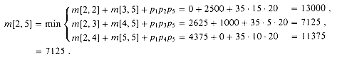
The m[i, j] values give the costs of optimal solutions to subproblems. To help us keep track of how to construct an optimal solution, let us define s[i, j] to be a value of k at which we can split the product AiAi+1 . . . Aj to obtain an optimal parenthesization. That is, s[i, j] equals a value k such that m[i, j] = m[i, k] + m[k + 1, j] + pi - 1pkpj .
At this point, it is a simple matter to write a recursive algorithm based on recurrence (16.2) to compute the minimum cost m[1, n] for multiplying A1A2 . . . An. As we shall see in Section 16.2, however, this algorithm takes exponential time--no better than the brute-force method of checking each way of parenthesizing the product.
The important observation that we can make at this point is that we have relatively few subproblems: one problem for each choice of i and j satisfying 1
Instead of computing the solution to recurrence (16.2) recursively, we perform the third step of the dynamic-programming paradigm and compute the optimal cost by using a bottom-up approach. The following pseudocode assumes that matrix Ai has dimensions pi - 1 X pi for i = 1, 2, . . . , n. The input is a sequence
The algorithm fills in the table m in a manner that corresponds to solving the parenthesization problem on matrix chains of increasing length. Equation (16.2)shows that the cost m[i, j] of computing a matrix-chain product of j - i + 1 matrices depends only on the costs of computing matrix-chain products of fewer than j - i + 1 matrices. That is, for k = i, i + 1, . . . ,j - 1, the matrix Ai..k is a product of k - i + 1 < j - i + 1 matrices and the matrix Ak+1 . . j a product of j - k < j - i + 1 matrices.
The algorithm first computes m[i, i]
Figure 16.1 illustrates this procedure on a chain of n = 6 matrices. Since we have defined m[i, j] only for i
The tables are rotated so that the main diagonal runs horizontally. Only the main diagonal and upper triangle are used in the m table, and only the upper triangle is used in the s table. The minimum number of scalar multiplications to multiply the 6 matrices is m[1, 6] = 15,125. Of the lightly shaded entries, the pairs that have the same shading are taken together in line 9 when computing
A simple inspection of the nested loop structure of MATRIX-CHAIN-ORDER yields a running time of O(n3) for the algorithm. The loops are nested three deep, and each loop index (l, i, and k) takes on at most n values. Exercise 16.1-3 asks you to show that the running time of this algorithm is in fact also
Although MATRIX-CHAIN-ORDER determines the optimal number of scalar multiplications needed to compute a matrix-chain product, it does not directly show how to multiply the matrices. Step 4 of the dynamic-programming paradigm is to construct an optimal solution from computed information.
In our case, we use the table s[1 . . n, 1 . . n] to determine the best way to multiply the matrices. Each entry s[i, j] records the value of k such that the optimal parenthesization of AiAi + 1
In the example of Figure 16.1, the call MATRIX-CHAIN-MULTIPLY(A, s, 1, 6) computes the matrix-chain product according to the parenthesization
16.1-1
Find an optimal parenthesization of a matrix-chain product whose sequence of dimensions is
16.1-2
Give an efficient algorithm PRINT-OPTIMAL-PARENS to print the optimal parenthesization of a matrix chain given the table s computed by MATRIX-CHAIN-ORDER. Analyze your algorithm.
16.1-3
Let R(i, j) be the number of times that table entry m[i, j] is referenced by MATRIX-CHAIN-ORDER in computing other table entries. Show that the total number of references for the entire table is
(Hint: You may find the identity
16.1-4
Show that a full parenthesization of an n-element expression has exactly n - 1 pairs of parentheses.
Although we have just worked through an example of the dynamic-programming method, you might still be wondering just when the method applies. From an engineering perspective, when should we look for a dynamic-programming solution to a problem? In this section, we examine the two key ingredients that an optimization problem must have for dynamic programming to be applicable: optimal substructure and overlapping subproblems. We also look at a variant method, called memoization, for taking advantage of the overlapping-subproblems property.
The first step in solving an optimization problem by dynamic programming is to characterize the structure of an optimal solution. We say that a problem exhibits optimal substructure if an optimal solution to the problem contains within it optimal solutions to subproblems. Whenever a problem exhibits optimal substructure, it is a good clue that dynamic programming might apply. (It also might mean that a greedy strategy applies, however. See Chapter 17.)
In Section 16.1, we discovered that the problem of matrix-chain multiplication exhibits optimal substructure. We observed that an optimal parenthesization of A1 A2
The optimal substructure of a problem often suggests a suitable space of subproblems to which dynamic programming can be applied. Typically, there are several classes of subproblems that might be considered "natural" for a problem. For example, the space of subproblems that we considered for matrix-chain multiplication contained all subchains of the input chain. We could equally well have chosen as our space of subproblems arbitrary sequences of matrices from the input chain, but this space of subproblems is unnecessarily large. A dynamic-programming algorithm based on this space of subproblems solves many more problems than it has to.
Investigating the optimal substructure of a problem by iterating on subproblem instances is a good way to infer a suitable space of subproblems for dynamic programming. For example, after looking at the structure of an optimal solution to a matrix-chain problem, we might iterate and look at the structure of optimal solutions to subproblems, subsubproblems, and so forth. We discover that all subproblems consist of subchains of
The second ingredient that an optimization problem must have for dynamic programming to be applicable is that the space of subproblems must be "small" in the sense that a recursive algorithm for the problem solves the same subproblems over and over, rather than always generating new subproblems. Typically, the total number of distinct subproblems is a polynomial in the input size. When a recursive algorithm revisits the same problem over and over again, we say that the optimization problem has overlapping subproblems. In contrast, a problem for which a divide-and-conquer approach is suitable usually generates brand-new problems at each step of the recursion. Dynamic-programming algorithms typically take advantage of overlapping subproblems by solving each subproblem once and then storing the solution in a table where it can be looked up when needed, using constant time per lookup.
To illustrate the overlapping-subproblems property, let us reexamine the matrix-chain multiplication problem. Referring back to Figure 16.1, observe that MATRIX-CHAIN-ORDER repeatedly looks up the solution to subproblems in lower rows when solving subproblems in higher rows. For example, entry m[3, 4] is referenced 4 times: during the computations of m[2, 4], m[1, 4], m[3, 5], and m[3, 6]. If m[3, 4] were recomputed each time, rather than just being looked up, the increase in running time would be dramatic. To see this, consider the following (inefficient) recursive procedure that determines m[i, j], the minimum number of scalar multiplications needed to compute the matrix-chain product Ai..j = AiAi + 1, . . . Aj. The procedure is based directly on the recurrence (16.2).
Figure 16.2 shows the recursion tree produced by the call RECURSIVE-MATRIX-CHAIN(p, 1, 4). Each node is labeled by the values of the parameters i and j. Observe that some pairs of values occur many times.
In fact, we can show that the running time T(n) to compute m[1, n] by this recursive procedure is at least exponential in n. Let us assume that the execution of lines 1-2 and of lines 6-7 each take at least unit time. Inspection of the procedure yields the recurrence
Noting that for i = 1, 2, . . . , n - 1, each term T(i) appears once as T(k) and once as T(n - k), and collecting the n - 1 1's in the summation together with the 1 out front, we can rewrite the recurrence as
We shall prove that T(n) =
which completes the proof. Thus, the total amount of work performed by the call RECURSIVE-MATRIX-CHAIN(p, 1, n) is at least exponential in n.
Compare this top-down, recursive algorithm with the bottom-up, dynamic-programming algorithm. The latter is more efficient because it takes advantage of the overlapping-subproblems property. There are only
There is a variation of dynamic programming that often offers the efficiency of the usual dynamic-programming approach while maintaining a top-down strategy. The idea is to memoize the natural, but inefficient, recursive algorithm. As in ordinary dynamic programming, we maintain a table with subproblem solutions, but the control structure for filling in the table is more like the recursive algorithm.
A memoized recursive algorithm maintains an entry in a table for the solution to each subproblem. Each table entry initially contains a special value to indicate that the entry has yet to be filled in. When the subproblem is first encountered during the execution of the recursive algorithm, its solution is computed and then stored in the table. Each subsequent time that the subproblem is encountered, the value stored in the table is simply looked up and returned.1
1This approach presupposes that the set of all possible subproblem parameters is known and that the relation between table positions and subproblems is established. Another approach is to memoize by using hashing with the subproblem parameters as keys.
The following procedure is a memoized version of RECURSIVE-MATRIX-CHAIN.
MEMOIZED-MATRIX-CHAIN, like MATRIX-CHAIN-ORDER, maintains a table m[1 . . n, 1 . . n] of computed values of m[i, j], the minimum number of scalar multiplications needed to compute the matrix Ai..j. Each table entry initially contains the value
Figure 16.2 illustrates how MEMOIZED-MATRIX-CHAIN saves time over RECURSIVE-MATRIX-CHAIN. Shaded subtrees represent values that are looked up rather than computed.
Like the dynamic-programming algorithm MATRIX-CHAIN-ORDER, the procedure MEMOIZED-MATRIX-CHAIN runs in O(n3 time. Each of
In summary, the matrix-chain multiplication problem can be solved in O(n3) time by either a top-down, memoized algorithm or a bottom-up, dynamic-programming algorithm. Both methods take advantage of the overlapping-subproblems property. There are only
In general practice, if all subproblems must be solved at least once, a bottom-up dynamic-programming algorithm usually outperforms a top-down memoized algorithm by a constant factor, because there is no overhead for recursion and less overhead for maintaining the table. Moreover, there are some problems for which the regular pattern of table accesses in the dynamic-programming algorithm can be exploited to reduce time or space requirements even further. Alternatively, if some subproblems in the subproblem space need not be solved at all, the memoized solution has the advantage of only solving those subproblems that are definitely required.
16.2-1
Compare the recurrence (16.4) with the recurrence (8.4) that arose in the analysis of the average-case running time of quicksort. Explain intuitively why the solutions to the two recurrences should be so dramatically different.
16.2-2
Which is a more efficient way to determine the optimal number of multiplications in a chain-matrix multiplication problem: enumerating all the ways of parenthesizing the product and computing the number of multiplications for each, or running RECURSIVE-MATRIX-CHAIN? Justify your answer.
16.2-3
Draw the recursion tree for the MERGE-SORT procedure from Section 1.3.1 on an array of 16 elements. Explain why memoization is ineffective in speeding up a good divide-and-conquer algorithm such as MERGE-SORT.
The next problem we shall consider is the longest-common-subsequence problem. A subsequence of a given sequence is just the given sequence with some elements (possibly none) left out. Formally, given a sequence X =
Given two sequences X and Y, we say that a sequence Z is a common subsequence of X and Y if Z is a subsequence of both X and Y. For example, if X =
In the longest-common-subsequence problem, we are given two sequences X =
A brute-force approach to solving the LCS problem is to enumerate all subsequences of X and check each subsequence to see if it is also a subsequence of Y, keeping track of the longest subsequence found. Each subsequence of X corresponds to a subset of the indices { 1, 2, . . . , m} of X. There are 2m subsequences of X, so this approach requires exponential time, making it impractical for long sequences.
The LCS problem has an optimal-substructure property, however, as the following theorem shows. As we shall see, the natural class of subproblems correspond to pairs of "prefixes" of the two input sequences. To be precise, given a sequence X =
Theorem 16.1
Let X =
1. If xm = yn, then zk = xm = yn and Zk-l is an LCS of Xm-l and Yn-l.
2. If xm
3. If xm
Proof (1) If zk
(2) If zk
(3) The proof is symmetric to (2).
The characterization of Theorem 16.1 shows that an LCS of two sequences contains within it an LCS of prefixes of the two sequences. Thus, the LCS problem has an optimal-substructure property. A recursive solution also has the overlapping-subproblems property, as we shall see in a moment.
Theorem 16.1 implies that there are either one or two subproblems to examine when finding an LCS of X =
We can readily see the overlapping-subproblems property in the LCS problem. To find an LCS of X and Y, we may need to find the LCS's of X and Yn-l and of Xm-l and Y. But each of these subproblems has the subsubproblem of finding the LCS of Xm-l and Yn-1. Many other subproblems share subsubproblems.
Like the matrix-chain multiplication problem, our recursive solution to the LCS problem involves establishing a recurrence for the cost of an optimal solution. Let us define c[i, j] to be the length of an LCS of the sequences Xi and Yj. If either i = 0 or j = 0, one of the sequences has length 0, so the LCS has length 0. The optimal substructure of the LCS problem gives the recursive formula
Based on equation (16.5), we could easily write an exponential-time recursive algorithm to compute the length of an LCS of two sequences. Since there are only
Procedure LCS-LENGTH takes two sequences X =
Figure 16.3 shows the tables produced by LCS-LENGTH on the sequences X =
The b table returned by LCS-LENGTH can be used to quickly construct an LCS of X =
For the b table in Figure 16.3, this procedure prints "BCBA" The procedure takes time O(m + n), since at least one of i and j is decremented in each stage of the recursion.
Once you have developed an algorithm, you will often find that you can improve on the time or space it uses. This is especially true of straightforward dynamic-programming algorithms. Some changes can simplify the code and improve constant factors but otherwise yield no asymptotic improvement in performance. Others can yield substantial asymptotic savings in time and space.
For example, we can eliminate the b table altogether. Each c[i, j] entry depends on only three other c table entries: c[i - 1,j - 1], c[i - 1,j], and c[i,j - 1]. Given the value of c[i,j], we can determine in O(1) time which of these three values was used to compute c[i,j], without inspecting table b. Thus, we can reconstruct an LCS in O(m + n) time using a procedure similar to PRINT-LCS. (Exercise 16.3-2 asks you to give the pseudocode.) Although we save
We can, however, reduce the asymptotic space requirements for LCS-LENGTH, since it needs only two rows of table c at a time: the row being computed and the previous row. (In fact, we can use only slightly more than the space for one row of c to compute the length of an LCS. See Exercise 16.3-4.) This improvement works if we only need the length of an LCS; if we need to reconstruct the elements of an LCS, the smaller table does not keep enough information to retrace our steps in O(m + n) time.
16.3-1
Determine an LCS of
16.3-2
Show how to reconstruct an LCS from the completed c table and the original sequences X =
16.3-3
Give a memoized version of LCS-LENGTH that runs in O(mn) time.
16.3-4
Show how to compute the length of an LCS using only 2 min(m, n) entries in the c table plus O(1) additional space. Then, show how to do this using min(m,n) entries plus O(1) additional space.
16.3-5
Give an O(n2)-time algorithm to find the longest monotonically increasing subsequence of a sequence of n numbers.
16.3-6
Give an O(n 1g n)-time algorithm to find the longest monotonically increasing subsequence of a sequence of n numbers. (Hint: Observe that the last element of a candidate subsequence of length i is at least as large as the last element of a candidate subsequence of length i - 1. Maintain candidate subsequences by linking them through the input sequence.)
In this section, we investigate the problem of optimally triangulating a convex polygon. Despite its outward appearance, we shall see that this geometric problem has a strong similarity to matrix-chain multiplication.
A polygon is a piecewise-linear, closed curve in the plane. That is, it is a curve ending on itself that is formed by a sequence of straight-line segments, called the sides of the polygon. A point joining two consecutive sides is called a vertex of the polygon. If the polygon is simple, as we shall generally assume, it does not cross itself. The set of points in the plane enclosed by a simple polygon forms the interior of the polygon, the set of points on the polygon itself forms its boundary, and the set of points surrounding the polygon forms its exterior. A simple polygon is convex if, given any two points on its boundary or in its interior, all points on the line segment drawn between them are contained in the polygon's boundary or interior.
We can represent a convex polygon by listing its vertices in counterclockwise order. That is, if P =
Given two nonadjacent vertices vi and vj, the segment
In the optimal (polygon) triangulation problem, we are given a convex polygon P =
where
There is a surprising correspondence between the triangulation of a polygon and the parenthesization of an expression such as a matrix-chain product. This correspondence is best explained using trees.
A full parenthesization of an expression corresponds to a full binary tree, sometimes called the parse tree of the expression. Figure 16.5(a) shows a parse tree for the parenthesized matrix-chain product
Each leaf of a parse tree is labeled by one of the atomic elements (matrices) in the expression. If the root of a subtree of the parse tree has a left subtree representing an expression El and a right subtree representing an expression Er, then the subtree itself represents the expression (ElEr). There is a one-to-one correspondence between parse trees and fully parenthesized expressions on n atomic elements.
A triangulation of a convex polygon
In recursive fashion, the polygon
In general, therefore, a triangulation of an n-sided polygon corresponds to a parse tree with n - 1 leaves. By an inverse process, one can produce a triangulation from a given parse tree. There is a one-to-one correspondence between parse trees and triangulations.
Since a fully parenthesized product of n matrices corresponds to a parse tree with n leaves, it therefore also corresponds to a triangulation of an (n + 1)-vertex polygon. Figures 16.5(a) and (b) illustrate this correspondence. Each matrix Ai in a product A1A2
In fact, the matrix-chain multiplication problem is a special case of the optimal triangulation problem. That is, every instance of matrix-chain multiplication can be cast as an optimal triangulation problem. Given a matrix-chain product A1A2
An optimal triangulation of P with respect to this weight function gives the parse tree for an optimal parenthesization of A1A2
Although the reverse is not true--the optimal triangulation problem is not a special case of the matrix-chain multiplication problem--it turns out that our code MATRIX-CHAIN-ORDER from Section 16.1, with minor modifications, solves the optimal triangulation problem on an (n + 1)- vertex polygon. We simply replace the sequence
After running the algorithm, the element m[1, n] contains the weight of an optimal triangulation. Let us see why this is so.
Consider an optimal triangulation T of an (n + 1)-vertex polygon P =
Just as we defined m[i, j] to be the minimum cost of computing the matrix-chain subproduct AiAi+1
Our next step is to define t[i, j] recursively. The basis is the degenerate case of a 2-vertex polygon: t[i, i] = 0 for i = 1, 2, . . . , n. When j - i
Compare this recurrence with the recurrence (16.2) that we developed for the minimum number m[i, j] of scalar multiplications needed to compute AiAi+1
16.4-1
Prove that every triangulation of an n-vertex convex polygon has n - 3 chords and divides the polygon into n - 2 triangles.
16.4-2
Professor Guinevere suggests that a faster algorithm to solve the optimal triangulation problem might exist for the special case in which the weight of a triangle is its area. Is the professor's intuition accurate?
16.4-3
Suppose that a weight function w is defined on the chords of a triangulation instead of on the triangles. The weight of a triangulation with respect to w is then the sum of the weights of the chords in the triangulation. Show that the optimal triangulation problem with weighted chords is just a special case of the optimal triangulation problem with weighted triangles.
16.4-4
Find an optimal triangulation of a regular octagon with unit-length sides. Use the weight function
where |vivj| is the euclidean distance from vi to vj. (A regular polygon is one with equal sides and equal interior angles.)
16-1 Bitonic euclidean traveling-salesman problem
The euclidean traveling-salesman problem is the problem of determining the shortest closed tour that connects a given set of n points in the plane. Figure 16.6(a) shows the solution to a 7-point problem. The general problem is NP-complete, and its solution is therefore believed to require more than polynomial time (see Chapter 36).
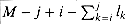
J. L. Bentley has suggested that we simplify the problem by restricting our attention to bitonic tours, that is, tours that start at the leftmost point, go strictly left to right to the rightmost point, and then go strictly right to left back to the starting point. Figure 16.6(b) shows the shortest bitonic tour of the same 7 points. In this case, a polynomial-time algorithm is possible.
Describe an O(n2)-time algorithm for determining an optimal bitonic tour. You may assume that no two points have the same x-coordinate. (Hint: Scan left to right, maintaining optimal possibilities for the two parts of the tour.)
16-2 Printing neatly
Consider the problem of neatly printing a paragraph on a printer. The input text is a sequence of n words of lengths l1,l2,...,ln, measured in characters. We want to print this paragraph neatly on a number of lines that hold a maximum of M characters each. Our criterion of "neatness" is as follows. If a given line contains words i through j and we leave exactly one space between words, the number of extra space characters at the end of the line is
16-3 Edit distance
When a "smart" terminal updates a line of text, replacing an existing "source" string x[1..m] with a new "target" string y[1..n], there are several ways in which the changes can be made. A single character of the source string can be deleted, replaced by another character, or copied to the target string; characters can be inserted; or two adjacent characters of the source string can be interchanged ("twiddled") while being copied to the target string. After all the other operations have occurred, an entire suffix of the source string can be deleted, an operation known as "kill to end of line."
As an example, one way to transform the source string algorithm to the target string altruistic is to use the following sequence of operations.
There are many other sequences of operations that accomplish the same result.
Each of the operations delete, replace, copy, insert, twiddle, and kill has an associated cost. (Presumably, the cost of replacing a character is less than the combined costs of deletion and insertion; otherwise, the replace operation would not be used.) The cost of a given sequence of transformation operations is the sum of the costs of the individual operations in the sequence. For the sequence above, the cost of converting algorithm to altruistic is
Given two sequences x[1..m] and y[1..n] and a given set of operation costs, the edit distance from x to y is the cost of the least expensive transformation sequence that converts x to y. Describe a dynamic-programming algorithm to find the edit distance from x[l..m] to y[1..n] and print an optimal transformation sequence. Analyze the running time and space requirements of your algorithm.
16-4 Planning a company party
Professor McKenzie is consulting for the president of A.-B. Corporation, which is planning a company party. The company has a hierarchical structure; that is, the supervisor relation forms a tree rooted at the president. The personnel office has ranked each employee with a conviviality rating, which is a real number. In order to make the party fun for all attendees, the president does not want both an employee and his or her immediate supervisor to attend.
a. Describe an algorithm to make up the guest list. The goal should be to maximize the sum of the conviviality ratings of the guests. Analyze the running time of your algorithm.
b. How can the professor ensure that the president gets invited to his own party?
16-5 Viterbi algorithm
We can use dynamic programming on a directed graph G = (V,E) for speech recognition. Each edge (u,v)
a. Describe an efficient algorithm that, given an edge-labeled graph G with distinguished vertex v0 and a sequence s =
Now, suppose that every edge (u,v)
b. Extend your answer to part (a) so that if a path is returned, it is a most probable path starting at v0 and having label s. Analyze the running time of your algorithm.
R. Bellman began the systematic study of dynamic programming in 1955. The word "programming," both here and in linear programming, refers to the use of a tabular solution method. Although optimization techniques incorporating elements of dynamic programming were known earlier, Bellman provided the area with a solid mathematical basis [21].
Hu and Shing [106] give an O(n 1g n)-time algorithm for the matrix-chain multiplication problem. They also demonstrate the correspondence between the optimal polygon triangulation problem and the matrix-chain multiplication problem.
The O(mn)-time algorithm for the longest-common-subsequence problem seems to be a folk algorithm. Knuth [43] posed the question of whether subquadratic algorithms for the LCS problem exist. Masek and Paterson [143] answered this question in the affirmative by giving an algorithm that runs in O(mn/lg n) time, where n
16.1 Matrix-chain multiplication
 A1, A2, . . ., An
 of n matrices to be multiplied, and we wish to compute the product
A1A2
 An .
An .(16.1)
A1, A2, A3, A4, the product A1A2A3A4 can be fully parenthesized in five distinct ways:(A1(A2(A3A4))) ,
(A1((A2A3)A4)) ,
((A1A2)(A3A4)) ,
((A1(A2A3))A4) ,
(((A1A2)A3)A4) .
MATRIX-MULTIPLY(A,B)
1 if columns [A]
 rows [B]
2 then error "incompatible dimensions"
3 else for i
 1 to rows [A]
4 do for j
1 to columns[B]5 do C[i, j]
06 for k
1 to columns [A]7 do C[i ,j]
C[i ,j] + A [i, k] B[k, j]8 return C
A1, A2, A3 of three matrices. Suppose that the dimensions of the matrices are 10 X 100,100  5, and 5 50, respectively. If we multiply according to the parenthesization ((A1A2)A3), we perform 10 100 5 = 5000 scalar multiplications to compute the 10 X 5 matrix product A1A2, plus another 10 5 50 = 2500 scalar multiplications to multiply this matrix by A3, for a total of 7500 scalar multiplications. If instead we multiply according to the parenthesization (A1(A2A3)), we perform 100 5 50 = 25,000 scalar multiplications to compute the 100 X 50 matrix product A2A3, plus another 10 100 50 = 50,000 scalar multiplications to multiply A1 by this matrix, for a total of 75,000 scalar multiplications. Thus, computing the product according to the first parenthesization is 10 times faster.A1, A2, . . . , An of n matrices, where for i = 1, 2, . . . , n , matrix Ai has dimension pi - 1 X pi, fully parenthesize the product A1 A2...An in a way that minimizes the number of scalar multiplications.
Counting the number of parenthesizations
P(n) = C (n - 1),
The structure of an optimal parenthesization
Aj. An optimal parenthesization of the product A1A2 An splits the product between Ak and Ak + 1 for some integer k in the range 1  k < n . That is, for some value of k, we first compute the matrices A1..k and Ak + 1..n and then multiply them together to produce the final product A1..n. The cost of this optimal parenthesization is thus the cost of computing the matrix A1..k, plus the cost of computing Ak + 1..n, plus the cost of multiplying them together. Ak within this optimal parenthesization of A1A2 An must be an optimal parenthesization of A1A2 Ak. Why? If there were a less costly way to parenthesize A1A2 Ak, substituting that parenthesization in the optimal parenthesization of A1A2 An would produce another parenthesization of A1A2 An whose cost was lower than the optimum: a contradiction. A similar observation holds for the the parenthesization of the subchain Ak+1Ak+2 An in the optimal parenthesization of A1A2 An: it must be an optimal parenthesization of Ak+1Ak+2 An.
A recursive solution
i j n. Let m[i, j] be the minimum number of scalar multiplications needed to compute the matrix Ai..j; the cost of a cheapest way to compute A1..n would thus be m[1, n]. k < j. Then, m[i, j] is equal to the minimum cost for computing the subproducts Ai..k and Ak+1..j, plus the cost of multiplying these two matrices together. Since computing the matrix product Ai..kAk+1..j takes pi-1pkpj scalar multiplications, we obtainm[i, j] = m[i, k] + m[k + 1, j] + pi-1pkpj .

(16.2)
Computing the optimal costs
i j n, or  + n =
+ n =  (n2) total. A recursive algorithm may encounter each subproblem many times in different branches of its recursion tree. This property of overlapping subproblems is the second hallmark of the applicability of dynamic programming.p0, p1, . . . , pn, here length[p] = n + 1. The procedure uses an auxiliary table m[1 . . n,1 . . n] for storing the m[i, j] costs and an auxiliary table s[1 . . n, 1 . . n] that records which index of k achieved the optimal cost in computing m[i, j].
MATRIX-CHAIN-ORDER(p)
1 n
length[p] - 12 for i
1 to n3 do m[i, i]
04 for l
2 to n5 do for i
1 to n - l + 16 do j
i + l-17 m[i, j]

8 for k
i to j - 19 do q
m[i, k] + m[k + 1, j] +pi - 1pkpj10 if q < m[i, j]
11 then m[i, j]
q12 s[i, j]
k13 return m and s
0 for i = 1, 2, . . . , n (the minimum costs for chains of length 1) in lines 2-3. It then uses recurrence (16.2) to compute m[i, i+ 1] for i = 1, 2, . . . , n - 1 (the minimum costs for chains of length l = 2) during the first execution of the loop in lines 4-12. The second time through the loop, it computes m[i, i + 2] for i = 1, 2, . . . , n - 2 (the minimum costs for chains of length l = 3), and so forth. At each step, the m[i, j] cost computed in lines 9-12 depends only on table entries m[i, k] and m[k + 1 ,j] already computed. j, only the portion of the table m strictly above the main diagonal is used. The figure shows the table rotated to make the main diagonal run horizontally. The matrix chain is listed along the bottom. Using this layout, the minimum cost m[i, j] for multiplying a subchain AiAi+1. . . Aj of matrices can be found at the intersection of lines running northeast from Ai and northwest from Aj. Each horizontal row in the table contains the entries for matrix chains of the same length. MATRIX-CHAIN-ORDER computes the rows from bottom to top and from left to right within each row. An entry m[i, j] is computed using the products pi - 1pkpj for k = i, i + 1, . . . , j - 1 and all entries southwest and southeast from m[i, j].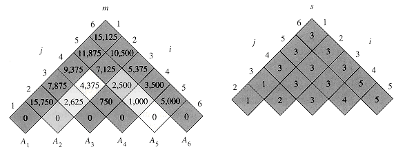
Figure 16.1 The m and s tables computed by MATRIX-CHAIN-ORDER for n = 6 and the following matrix dimensions:
matrix dimension
-----------------
A1 30 X 35
A2 35 X 15
A3 15 X 5
A4 5 X 10
A5 10 X 20
A6 20 X 25
 (n3). The algorithm requires (n2) space to store the m and s tables. Thus, MATRIX-CHAIN-ORDER is much more efficient than the exponential-time method of enumerating all possible parenthesizations and checking each one.
Constructing an optimal solution
Aj splits the product between Ak and Ak + 1. Thus, we know that the final matrix multiplication in computing A1..n optimally is A1..s[1,n]As[1,n]+1..n. The earlier matrix multiplications can be computed recursively, since s[l,s[1,n]] determines the last matrix multiplication in computing A1..s[1,n], and s[s[1,n] + 1, n] determines the last matrix multiplication in computing As[1,n]+..n. The following recursive procedure computes the matrix-chain product Ai..j given the matrices A = A1, A2, . . . , An, the s table computed by MATRIX-CHAIN-ORDER, and the indices i and j. The initial call is MATRIX-CHAIN-MULTIPLY(A, s, 1, n).MATRIX-CHAIN-MULTIPLY(A, s, i, ,j)
1 if j >i
2 then X
MATRIX-CHAIN-MULTIPLY(A, s, i, s[i, j])3 Y
MATRIX-CHAIN-MULTIPLY(A, s, s[i, j] + 1, j)4 return MATRIX-MULTIPLY(X, Y)
5 else return Ai
((A1(A2A3))((A4A5)A6)) .
(16.3)
Exercises
5, 10, 3, 12, 5, 50, 6.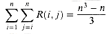
16.2 Elements of dynamic programming
Optimal substructure
An that splits the product between Ak and Ak + 1 contains within it optimal solutions to the problems of parenthesizing A1A2 A k and Ak + 1Ak + 2. . . An. The technique that we used to show that subproblems have optimal solutions is typical. We assume that there is a better solution to the subproblem and show how this assumption contradicts the optimality of the solution to the original problem.Al, A2, . . . , An. Thus, the set of chains of the form Ai, Aj+l, . . . , Aj for 1 i j n makes a natural and reasonable space of subproblems to use.Overlapping subproblems
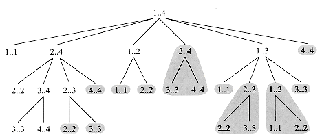
Figure 16.2 The recursion tree for the computation of RECURSIVE-MATRIX-CHAIN(p, 1, 4). Each node contains the parameters i and j. The computations performed in a shaded subtree are replaced by a single table lookup in MEMOIZED-MATRIX-CHAIN(p, 1, 4).
RECURSIVE-MATRIX-CHAIN(p, i, j)
1 if i = j
2 then return 0
3 m[i, j]
4 for k
i to j - 15 do q
RECURSIVE-MATRIX-CHAIN(p, i, k)+ RECURSIVE-MATRIX-CHAIN(p, k + 1, j) + pi-1pkpj
6 if q < m[i, j]
7 then m[i, j]
q8 return m[i, j]

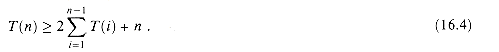
(16.4)
(2n) using the substitution method. Specifically, we shall show that T(n)  2n-1 for all n > 1. The basis is easy, since T(1) > 1 = 2
 . Inductively, for n 2 we have
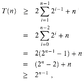 (n2) different subproblems, and the dynamic-programming algorithm solves each exactly once. The recursive algorithm, on the other hand, must repeatedly resolve each subproblem each time it reappears in the recursion tree. Whenever a recursion tree for the natural recursive solution to a problem contains the same subproblem repeatedly, and the total number of different subproblems is small, it is a good idea to see if dynamic programming can be made to work.
Memoization
MEMOIZED-MATRIX-CHAIN(p)
1 n
length[p] - 12 for i
1 to n3 do for j
i to n4 do m[i, j]
5 return LOOKUP-CHAIN(p, 1, n)
LOOKUP-CHAIN(p, i, j)
1 if m[i,j] <
2 then return m[i, j]
3 if i = j
4 then m[i, j]
05 else for k
i to j - 16 do q
LOOKUP-CHAIN(p, i, k)+ LOOKUP-CHAIN(p, k + 1, j) + pi - 1pkpj
7 if q < m[i, j]
8 then m[i, j]
q9 return m[i, j]
to indicate that the entry has yet to be filled in. When the call LOOKUP-CHAIN(p, i, j) is executed, if m[i, j] < in line 1, the procedure simply returns the previously computed cost m[i, j] (line 2). Otherwise, the cost is computed as in RECURSIVE-MATRIX-CHAIN, stored in m[i, j], and returned. (The value is convenient to use for an unfilled table entry since it is the value used to initialize m[i, j] in line 3 of RECURSIVE-MATRIX-CHAIN.) Thus, LOOKUP-CHAIN(p, i, j) always returns the value of m[i, j], but it only computes it if this is the first time that LOOKUP-CHAIN has been called with the parameters i and j.(n2) table entries is initialized once in line 4 of MEMOIZED-MATRIX-CHAIN and filled in for good by just one call of LOOKUP-CHAIN. Each of these (n2) calls to LOOKUP-CHAIN takes O(n) time, excluding the time spent in computing other table entries, so a total of O(n3) is spent altogether. Memoization thus turns an (2n) algorithm into an O(n3) algorithm.(n2) different subproblems in total, and either of these methods computes the solution to each subproblem once. Without memoization, the natural recursive algorithm runs in exponential time, since solved subproblems are repeatedly solved.Exercises
16.3 Longest common subsequence
x1, x2, . . . , xm, another sequence Z = z1, z2, . . . , zk is a subsequence of X if there exists a strictly increasing sequence i1, i2, . . . , ik of indices of X such that for all j = 1, 2, . . . , k, we have xij = zj. For example, Z = B, C, D, B is a subsequence of X = A, B, C, B, D, A, B with corresponding index sequence 2, 3, 5, 7.A, B, C, B, D, A, B and Y = B, D, C, A, B, A, the sequence B, C, A is a common subsequence of both X and Y. The sequence B, C, A is not a longest common subsequence LCS of X and Y, however, since it has length 3 and the sequence B, C, B, A, which is also common to both X and Y, has length 4. The sequence B, C, B, A is an LCS of X and Y, as is the sequence B, D, A, B, since there is no common subsequence of length 5 or greater.x1, x2, . . . , xm and Y = y1, y2, . . . , yn and wish to find a maximum-length common subsequence of X and Y. This section shows that the LCS problem can be solved efficiently using dynamic programming.Characterizing a longest common subsequence
x1, x2, . . . ,xm, we define the ith prefix of X, for i = 0, 1,...,m, as Xi = x1, x2, . . . , xi. For example, if X = A, B, C, B, D, A, B, then X4 = A, B, C, B and X0 is the empty sequence.x1, x2, . . . , xm and Y = y1, y2, . . . , yn be sequences, and let Z = z1, z2, . . . , zk be any LCS of X and Y. yn, then zk xm implies that Z is an LCS of Xm-1 and Y. yn, then zk yn implies that Z is an LCS of X and Yn-l. xm, then we could append xm = yn to Z to obtain a common subsequence of X and Y of length k + 1, contradicting the supposition that Z is a longest common subsequence of X and Y. Thus, we must have zk = xm = yn. Now, the prefix Zk-l is a length-(k - 1)common subsequence of Xm-1 and Yn-l. We wish to show that it is an LCS. Suppose for the purpose of contradiction that there is a common subsequence W of Xm-l and Yn-l with length greater than k - 1. Then, appending xm = yn to W produces a common subsequence of X and Y whose length is greater than k, which is a contradiction. xm, then Z is a common subsequence of Xm-1 and Y. If there were a common subsequence W of Xm-l and Y with length greater than k, then W would also be a common subsequence of Xm and Y, contradicting the assumption that Z is an LCS of X and Y.A recursive solution to subproblems
x1, x2, . . . , xm and Y = y1, y2, . . . , yn. If xm = yn we must find an LCS of Xm-l and Yn-l. Appending xm = yn, to this LCS yields an LCS of X and Y. If xm yn, then we must solve two subproblems: finding an LCS of Xm-l and Y and finding an LCS of X and Yn-1. Whichever of these two LCS's is longer is an LCS of X and Y.
(16.5)
Computing the length of an LCS
(mn) distinct subproblems, however, we can use dynamic programming to compute the solutions bottom up.x1,x2,...,xm and Y = y1,y2,...,yn as inputs. It stores the c[i, j] values in a table c[0 . . m, 0 . . n] whose entries are computed in row-major order. (That is, the first row of c is filled in from left to right, then the second row, and so on.) It also maintains the table b[1 . . m, 1 . . n] to simplify construction of an optimal solution. Intuitively, b[i, j] points to the table entry corresponding to the optimal subproblem solution chosen when computing c[i, j]. The procedure returns the b and c tables; c[m, n] contains the length of an LCS of X and Y.LCS-LENGTH(X,Y)
1 m
length[X]2 n
length[Y]3 for i
1 to m4 do c[i,0]
05 for j
0 to n6 do c[0, j]
07 for i
1 to m8 do for j
1 to n9 do if xi = yj
10 then c[i, j]
c[i - 1, j -1] + 111 b[i, j]
" "
"12 else if c[i - 1, j]
c[i, j - 1]13 then c[i, j]
c[i - 1, j]14 b[i, j]
" "
"15 else c[i, j]
c[i, j -1]16 b[i, j]
""17 return c and b
A, B, C, B, D, A, B and Y = B, D, C, A, B, A. The running time of the procedure is O(mn), since each table entry takes O(1) time to compute.Constructing an LCS
x1,x2,...,xm) and Y = y1,y2,...,yn). We simply begin at b[m, n] and trace through the table following the arrows. Whenever we encounter a " in entry b[i,j], it implies that xi = yj is an element of the LCS. The elements of the LCS are encountered in reverse order by this method. The following recursive procedure prints out an LCS of X and Y in the proper, forward order. The initial invocation is PRINT-LCS(b, X, length[X], length[Y]).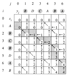
Figure 16.3 The c and b tables computed by LCS-LENGTH on the sequences X =
A, B, C, B, D, A, B and Y = B, D, C, A, B, A. The square in row i and column j contains the value of c[i, j] and the appropriate arrow for the value of b[i, j]. The entry 4 in c[7, 6]--the lower right-hand corner of the table--is the length of an LCS B, C, B, A of X and Y. For i, j > 0, entry c[i, j] depends only on whether xi = yj and the values in entries c[i -1, j], c[i, j - 1], and c[i - 1, j - 1], which are computed before c[i, j]. To reconstruct the elements of an LCS, follow the b[i, j] arrows from the lower right-hand corner; the path is shaded. Each " on the path corresponds to an entry (highlighted) for which xi = yj is a member of an LCS.PRINT-LCS(b,X,i,j)
1 if i = 0 or j = 0
2 then return
3 if b[i, j] = "
"4 then PRINT-LCS(b,X,i - 1, j - 1)
5 print xi
6 elseif b[i,j] = "
"7 then PRINT-LCS(b,X,i - 1,j)
8 else PRINT-LCS(b,X,i, j - 1)
Improving the code
(mn) space by this method, the auxiliary space requirement for computing an LCS does not asymptotically decrease, since we need (mn) space for the c table anyway.Exercises
1,0,0,1,0,1,0,1 and 0,1,0,1,1,0,1,1,0.x1,x2,...,xm and Y = y1,y2,...,yn in O(m + n) time, without using the b table.16.4 Optimal polygon triangulation
v0,v1,...,vn-1 is a convex polygon, it has n sides  , where we interpret vn as v0. (In general, we shall implicitly assume arithmetic on vertex indices is taken modulo the number of vertices.)
 is a chord of the polygon. A chord
  divides the polygon into two polygons: vi,vi+1,...,vj and vj,vj+1,...,vi. A triangulation of a polygon is a set T of chords of the polygon that divide the polygon into disjoint triangles (polygons with 3 sides). Figure 16.4 shows two ways of triangulating a 7-sided polygon. In a triangulation, no chords intersect (except at endpoints) and the set T of chords is maximal: every chord not in T intersects some chord in T. The sides of triangles produced by the triangulation are either chords in the triangulation or sides of the polygon. Every triangulation of an n-vertex convex polygon has n - 3 chords and divides the polygon into n - 2 triangles.v0, v1,...,vn-1 and a weight function w defined on triangles formed by sides and chords of P. The problem is to find a triangulation that minimizes the sum of the weights of the triangles in the triangulation. One weight function on triangles that comes to mind naturally is
 vivj is the euclidean distance from vi to vj. The algorithm we shall develop works for an arbitrary choice of weight function.
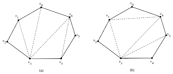
Figure 16.4 Two ways of triangulating a convex polygon. Every triangulation of this 7-sided polygon has 7 - 3 = 4 chords and divides the polygon into 7 - 2 = 5 triangles.
Correspondence to parenthesization
((A1(A2A3))(A4(A5A6))) .
(16.6)
v0, v1, . . . , vn - 1 can also be represented by a parse tree. Figure 16.5(b) shows the parse tree for the triangulation of the polygon from Figure 16.4(a). The internal nodes of the parse tree are the chords of the triangulation plus the side  , which is the root. The leaves are the other sides of the polygon. The root
  is one side of the triangle
  . This triangle determines the children of the root: one is the chord
  , and the other is the chord
  . Notice that this triangle divides the original polygon into three parts: the triangle
  itself, the polygon v0, v1, . . . , v3, and the polygon v3, v4, . . . , v6. Moreover, the two subpolygons are formed entirely by sides of the original polygon, except for their roots, which are the chords
  and
and  .
.
Figure 16.5 Parse trees. (a) The parse tree for the parenthesized product ((A1(A2A3))(A4(A5A6))) and for the triangulation of the 7-sided polygon from Figure 16.4(a). (b) The triangulation of the polygon with the parse tree overlaid. Each matrix Ai corresponds to the side
 for i = 1, 2, . . . , 6.v0, v1, . . . , v3 contains the left subtree of the root of the parse tree, and the polygon v3, v4, . . . , v6 contains the right subtree. An corresponds to a side
  of an (n + 1)-vertex polygon. A chord
  , where i < j, corresponds to a matrix Ai+1..j computed during the evaluation of the product. An, we define an (n + 1)-vertex convex polygon P = v0, v1, . . . , vn. If matrix Ai has dimensions pi-1 pi for i = 1, 2, . . . , n, we define the weight function for the triangulation as
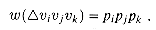 An.p0, p1, . . . , pn of matrix dimensions with the sequence v0, v1, . . . , vn of vertices, change references to p to references to v, and change line 9 to read:
The substructure of an optimal triangulation
v0, v1, . . . , vn that includes the triangle  for some k, where 1 k n - 1. The weight of T is just the sum of the weights of
  and triangles in the triangulation of the two subpolygons v0, v1, . . . , vk and vk, vk+1, . . . , vn. The triangulations of the subpolygons determined by T must therefore be optimal, since a lesser-weight triangulation of either subpolygon would contradict the minimality of the weight of T.
A recursive solution
Aj, let us define t[i, j], for 1 i < j n, to be the weight of an optimal triangulation of the polygon vi - 1, v1 . . . , vj. For convenience, we consider a degenerate polygon vi - 1, vi to have weight 0. The weight of an optimal triangulation of polygon P is given by t[1, n]. 1, we have a polygon vi - 1, vi, . . . , vj with at least 3 vertices. We wish to minimize over all vertices vk, for k = i, i + 1, . . . , j - 1, the weight of  plus the weights of the optimal triangulations of the polygons vi - 1, vi, . . . , vk and vk, vk+1, . . . , vj. The recursive formulation is thus
(16.7)
Aj. Except for the weight function, the recurrences are identical, and thus, with the minor changes to the code mentioned above, the procedure MATRIX-CHAIN-ORDER can compute the weight of an optimal triangulation. Like MATRIX-CHAIN-ORDER, the optimal triangulation procedure runs in time (n3) and uses (n2) space.Exercises
Problems
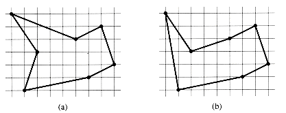
Figure 16.6 Seven points in the plane, shown on a unit grid. (a) The shortest closed tour, with length 24.88 . . .. This tour is not bitonic. (b) The shortest bitonic tour for the same set of points. Its length is 25.58 . . ..
 We wish to minimize the sum, over all lines except the last, of the cubes of the numbers of extra space characters at the ends of lines. Give a dynamic-programming algorithm to print a paragraph of n words neatly on a printer. Analyze the running time and space requirements of your algorithm.
Operation Target string Source string
------------------------------------------------
copy a a lgorithm
copy l al gorithm
replace g by t alt orithm
delete o alt rithm
copy r altr ithm
insert u altru ithm
insert i altrui ithm
insert s altruis ithm
twiddle it into ti altruisti hm
insert c altruistic hm
kill hm altruistic
(3 cost(copy)) + cost(replace) + cost(delete) + (3 cost(insert))
+ cost(twiddle) + cost(kill) .
 E is labeled with a sound
  (u,v) from a finite set of sounds. The labeled graph is a formal model of a person speaking a restricted language. Each path in the graph starting from a distinguished vertex v0 V corresponds to a possible sequence of sounds produced by the model. The label of a directed path is defined to be the concatenation of the labels of the edges on that path.1,2,...,k of characters from , returns a path in G that begins at v0 and has s as its label, if any such path exists. Otherwise, the algorithm should return NO-SUCH-PATH. Analyze the running time of your algorithm. (Hint: You may find concepts from Chapter 23 useful.) E has also been given an associated nonnegative probability p(u, v) of traversing the edge (u, v) from vertex u and producing the corresponding sound. The sum of the probabilities of the edges leaving any vertex equals 1. The probability of a path is defined to be the product of the probabilities of its edges. We can view the probability of a path beginning at v0 as the probability that a "random walk" beginning at v0 will follow the specified path, where the choice of which edge to take at a vertex u is made probabilistically according to the probabilities of the available edges leaving u.
Chapter notes
m and the sequences are drawn from a set of bounded size. For the special case in which no element appears more than once in an input sequence, Szymanski [184] shows that the problem can be solved in O((n+m) lg(n+m)) time. Many of these results extend to the problem of computing string edit distances (Problem 16-3).