


Some applications involve grouping n distinct elements into a collection of disjoint sets. Two important operations are then finding which set a given element belongs to and uniting two sets. This chapter explores methods for maintaining a data structure that supports these operations.
Section 22.1 describes the operations supported by a disjoint-set data structure and presents a simple application. In Section 22.2, we look at a simple linked-list implementation for disjoint sets. A more efficient representation using rooted trees is given in Section 22.3. The running time using the tree representation is linear for all practical purposes but is theoretically superlinear. Section 22.4 defines and discusses Ackermann's function and its very slowly growing inverse, which appears in the running time of operations on the tree-based implementation, and then uses amortized analysis to prove a slightly weaker upper bound on the running time.
A disjoint-set data structure maintains a collection S = {S1, S2, . . . ,Sk} of disjoint dynamic sets. Each set is identified by a representative, which is some member of the set. In some applications, it doesn't matter which member is used as the representative; we only care that if we ask for the representative of a dynamic set twice without modifying the set between the requests, we get the same answer both times. In other applications, there may be a prespecified rule for choosing the representative, such as choosing the smallest member in the set (assuming, of course, that the elements can be ordered).
As in the other dynamic-set implementations we have studied, each element of a set is represented by an object. Letting x denote an object, we wish to support the following operations.
MAKE-SET(x) creates a new set whose only member (and thus representative) is pointed to by x. Since the sets are disjoint, we require that x not already be in a set.
UNION(x, y) unites the dynamic sets that contain x and y, say Sx and Sy, into a new set that is the union of these two sets. The two sets are assumed to be disjoint prior to the operation. The representative of the resulting set is some member of Sx
FIND-SET(x) returns a pointer to the representative of the (unique) set containing x.
Throughout this chapter, we shall analyze the running times of disjoint-set data structures in terms of two parameters: n, the number of MAKE-SET operations, and m, the total number of MAKE-SET, UNION, and FIND-SET operations. Since the sets are disjoint, each UNION operation reduces the number of sets by one. After n - 1 UNION operations, therefore, only one set remains. The number of UNION operations is thus at most n - 1. Note also that since the MAKE-SET operations are included in the total number of operations m, we have m
One of the many applications of disjoint-set data structures arises in determining the connected components of an undirected graph (see Section 5.4). Figure 22.1(a), for example, shows a graph with four connected components.
The procedure CONNECTED-COMPONENTS that follows uses the disjoint-set operations to compute the connected components of a graph. Once CONNECTED-COMPONENTS has been run as a preprocessing step, the procedure SAME-COMPONENT answers queries about whether two vertices are in the same connected component.1 (The set of vertices of a graph G is denoted by V[G], and the set of edges is denoted by E[G].)
1When the edges of the graph are "static"--not changing over time--the connected components can be computed faster by using depth-first search (Exercise 23.3-9). Sometimes, however, the edges are added "dynamically" and we need to maintain the connected components as each edge is added. In this case, the implementation given here can be more efficient than running a new depth-first search for each new edge.
The procedure CONNECTED-COMPONENTS initially places each vertex v in its own set. Then, for each edge (u, v), it unites the sets containing u and v. By Exercise 22.1-2, after all the edges are processed, two vertices are in the same connected component if and only if the corresponding objects are in the same set. Thus, CONNECTED-COMPONENTS computes sets in such a way that the procedure SAME-COMPONENT can determine whether two vertices are in the same connected component. Figure 22.1 (b) illustrates how the disjoint sets are computed by CONNECTED-COMPONENTS.
22.1-1
Suppose that CONNECTED-COMPONENTS is run on the undirected graph G = (V, E), where V = {a, b, c, d, e, f, g, h, i, j, k} and the edges of E are processed in the following order: (d, i), (f, k), (g, i), (b, g), (a, h), (i, j), (d, k), (b, j), (d, f), (g, j), (a, e), (i, d). List the vertices in each connected component after each iteration of lines 3-5.
22.1-2
Show that after all edges are processed by CONNECTED-COMPONENTS, two vertices are in the same connected component if and only if they are in the same set.
22.1-3
During the execution of CONNECTED-COMPONENTS on an undirected graph G = (V, E) with k connected components, how many times is FIND-SET called? How many times is UNION called? Express your answers in terms of |V|, |E|, and k.
A simple way to implement a disjoint-set data structure is to represent each set by a linked list. The first object in each linked list serves as its set's representative. Each object in the linked list contains a set member, a pointer to the object containing the next set member, and a pointer back to the representative. Figure 22.2(a) shows two sets. Within each linked list, the objects may appear in any order (subject to our assumption that the first object in each list is the representative).
With this linked-list representation, both MAKE-SET and FIND-SET are easy, requiring O(1) time. To carry out MAKE-SET(x), we create a new linked list whose only object is x. For FIND-SET(x), we just return the pointer from x back to the representative.
The simplest implementation of the UNION operation using the linked-list set representation takes significantly more time than MAKE-SET or FIND-SET. As Figure 22.2(b) shows, we perform UNION(x, y) by appending x's list onto the end of y's list. The representative of the new set is the element that was originally the representative of the set containing y. Unfortunately, we must update the pointer to the representative for each object originally on x's list, which takes time linear in the length of x's list.
In fact, it is not difficult to come up with a sequence of m operations that requires
The total time spent is therefore
The above implementation of the UNION procedure requires an average of
Theorem 22.1
Using the linked-list representation of disjoint sets and the weighted-union heuristic, a sequence of m MAKE-SET, UNION, and FIND-SET operations, n of which are MAKE-SET operations, takes O(m + n 1g n) time.
Proof We start by computing, for each object in a set of size n, an upper bound on the number of times the object's pointer back to the representative has been updated. Consider a fixed object x. We know that each time x's representative pointer was updated, x must have started in the smaller set. The first time x's representative pointer was updated, therefore, the resulting set must have had at least 2 members. Similarly, the next time x's representative pointer was updated, the resulting set must have had at least 4 members. Continuing on, we observe that for any k
The time for the entire sequence of m operations follows easily. Each MAKE-SET and FIND-SET operation takes O(1) time, and there are O(m) of them. The total time for the entire sequence is thus O(m + n 1g n).
22.2-1
Write pseudocode for MAKE-SET, FIND-SET, and UNION using the linked-list representation and the weighted-union heuristic. Assume that each object x has attributes rep[x] pointing to the representative of the set containing x, last[x] pointing to the last object in the linked list containing x, and size[x] giving the size of the set containing x. Your pseudocode can assume that last[x] and size[x] are correct only if x is a representative.
22.2-2
Show the data structure that results and the answers returned by the FIND-SET operations in the following program. Use the linked-list representation with the weighted-union heuristic.
22.2-3
Argue on the basis of Theorem 22.1 that we can obtain amortized time bounds of O(1) for MAKE-SET and FIND-SET and O(1g n) for UNION using the linked-list representation and the weighted-union heuristic.
22.2-4
Give a tight asymptotic bound on the running time of the sequence of operations in Figure 22.3 assuming the linked-list representation and the weighted-union heuristic.
In a faster implementation of disjoint sets, we represent sets by rooted trees, with each node containing one member and each tree representing one set. In a disjoint-set forest, illustrated in Figure 22.4(a), each member points only to its parent. The root of each tree contains the representative and is its own parent. As we shall see, although the straightforward algorithms that use this representation are no faster than ones that use the linked-list representation, by introducing two heuristics--"union by rank" and "path compression"--we can achieve the asymptotically fastest disjoint-set data structure known.
We perform the three disjoint-set operations as follows. A MAKE-SET operation simply creates a tree with just one node. We perform a FIND-SET operation by chasing parent pointers until we find the root of the tree. The nodes visited on this path toward the root constitute the find path. A UNION operation, shown in Figure 22.4(b), causes the root of one tree to point to the root of the other.
So far, we have not improved on the linked-list implementation. A sequence of n - 1 UNION operations may create a tree that is just a linear chain of n nodes. By using two heuristics, however, we can achieve a running time that is almost linear in the total number of operations m.
The first heuristic, union by rank, is similar to the weighted-union heuristic we used with the linked-list representation. The idea is to make the root of the tree with fewer nodes point to the root of the tree with more nodes. Rather than explicitly keeping track of the size of the subtree rooted at each node, we shall use an approach that eases the analysis. For each node, we maintain a rank that approximates the logarithm of the subtree size and is also an upper bound on the height of the node. In union by rank, the root with smaller rank is made to point to the root with larger rank during a UNION operation.
The second heuristic, path compression, is also quite simple and very effective. As shown in Figure 22.5, we use it during FIND-SET operations to make each node on the find path point directly to the root. Path compression does not change any ranks.
To implement a disjoint-set forest with the union-by-rank heuristic, we must keep track of ranks. With each node x, we maintain the integer value rank[x], which is an upper bound on the height of x (the number of edges in the longest path between x and a descendant leaf). When a singleton set is created by MAKE-SET, the initial rank of the single node in the corresponding tree is 0. Each FIND-SET operation leaves all ranks unchanged. When applying UNION to two trees, we make the root of higher rank the parent of the root of lower rank. In case of a tie, we arbitrarily choose one of the roots as the parent and increment its rank.
Let us put this method into pseudocode. We designate the parent of node x by p[x]. The LINK procedure, a subroutine called by UNION, takes pointers to two roots as inputs.
The FIND-SET procedure with path compression is quite simple.
The FIND-SET procedure is a two-pass method: it makes one pass up the find path to find the root, and it makes a second pass back down the find path to update each node so that it points directly to the root. Each call of FIND-SET(x) returns p[x] in line 3. If x is the root, then line 2 is not executed and p[x] = x is returned. This is the case in which the recursion bottoms out. Otherwise, line 2 is executed, and the recursive call with parameter p[x] returns a pointer to the root. Line 2 updates node x to point directly to the root, and this pointer is returned in line 3.
Separately, either union by rank or path compression improves the running time of the operations on disjoint-set forests, and the improvement is even greater when the two heuristics are used together. Alone, union by rank yields the same running time as we achieved with the weighted union heuristic for the list representation: the resulting implementation runs in time O(m lg n) (see Exercise 22. 4-3). This bound is tight (see Exercise 22.3-3). Although we shall not prove it here, if there are n MAKE-SET operations (and hence at most n - 1 UNION operations) and â FIND-SET operations, the path-compression heuristic alone gives a worst-case running time of
When we use both union by rank and path compression, the worst-case running time is O(m
22.3-1
Do Exercise 22.2-2 using a disjoint-set forest with union by rank and path compression.
22.3-2
Write a nonrecursive version of FIND-SET with path compression.
22.3-3
Give a sequence of m MAKE-SET, UNION, and FIND-SET operations, n of which are MAKE-SET operations, that takes
22.3-4
Show that any sequence of m MAKE-SET, FIND-SET, and UNION operations, where all the UNION operations appear before any of the FIND-SET operations, takes only O(m) time if both path compression and union by rank are used. What happens in the same situation if only the path-compression heuristic is used?
As noted in Section 22.3, the running time of the combined union-by-rank and path-compression heuristic is O(m
To understand Ackermann's function and its inverse
stands for the function g(i), defined recursively by
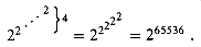
Intuitively, the parameter i gives the "height of the stack of 2's" that make up the exponent. For example,
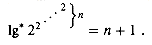
Recall the definition of the function 1g* in terms of the functions lg(i) defined for integer i
The 1g* function is essentially the inverse of repeated exponentiation:
We are now ready to show Ackermann's function, which is defined for integers i, j
Figure 22.6 shows the value of the function for small values of i and j.
Figure 22.7 shows schematically why Ackermann's function has such explosive growth. The first row, exponential in the column number j, is already rapidly growing. The second row consists of the widely spaced subset of columns
We define the inverse of Ackermann's function by2
2Although this function is not the inverse of Ackermann's function in the true mathematical sense, it captures the spirit of the inverse in its growth, which is as slow as Ackermann's function is fast. The reason we use the mysterious lg n threshold is revealed in the proof of the O(m
If we fix a value of n, then as m increases, the function
To back up our earlier claim that
which is far greater than the estimated number of atoms in the observable universe (roughly 1080). It is only for impractically large values of n that A(4, 1)
In the remainder of this section, we prove an O(m 1g* n) bound on the running time of the disjoint-set operations with union by rank and path compression. In order to prove this bound, we first prove some simple properties of ranks.
Lemma 22.2
For all nodes x, we have rank[x]
Proof The proof is a straightforward induction on the number of operations, using the implementations of MAKE-SET, UNION, and FIND-SET that appear in Section 22.3. We leave it as Exercise 22.4-1.
We define size(x) to be the number of nodes in the tree rooted at node x, including node x itself.
Lemma 22.3
For all tree roots x, size(x)
Proof The proof is by induction on the number of LINK operations. Note that FIND-SET operations change neither the rank of a tree root nor the size of its tree.
Basis: The lemma is true before the first LINK, since ranks are initially 0 and each tree contains at least one node.
Inductive step: Assume that the lemma holds before performing the operation LINK(x, y). Let rank denote the rank just before the LINK, and let rank' denote the rank just after the LINK. Define size and size' similarly.
If rank[x]
No ranks or sizes change for any nodes other than y.
If rank[x] = rank[y], node y is again the root of the new tree, and
Lemma 22.4
For any integer r
Proof Fix a particular value of r. Suppose that when we assign a rank r to a node x (in line 2 of MAKE-SET or in line 5 of LINK), we attach a label x to each node in the tree rooted at x. By Lemma 22.3, at least 2r nodes are labeled each time. Suppose that the root of the tree containing node x changes. Lemma 22.2 assures us that the rank of the new root (or, in fact, of any proper ancestor of x) is at least r + 1. Since we assign labels only when a root is assigned a rank r, no node in this new tree will ever again be labeled. Thus, each node is labeled at most once, when its root is first assigned rank r. Since there are n nodes, there are at most n labeled nodes, with at least 2r labels assigned for each node of rank r. If there were more than n/2r nodes of rank r, then more than 2r. (n/2r) = n nodes would be labeled by a node of rank r, which is a contradiction. Therefore, at most n/2r nodes are ever assigned rank r.
Corollary 22.5
Every node has rank at most
Proof If we let r > 1g n, then there are at most n/2r < 1 nodes of rank r. Since ranks are natural numbers, the corollary follows.
We shall use the aggregate method of amortized analysis (see Section 18.1) to prove the O(m 1g* n) time bound. In performing the amortized analysis, it is convenient to assume that we invoke the LINK operation rather than the UNION operation. That is, since the parameters of the LINK procedure are pointers to two roots, we assume that the appropriate FIND-SET operations are performed if necessary. The following lemma shows that even if we count the extra FIND-SET operations, the asymptotic running time remains unchanged.
Lemma 22.6
Suppose we convert a sequence S' of m' MAKE-SET, UNION, and FIND-SET operations into a sequence S of m MAKE-SET, LINK, and FIND-SET operations by turning each UNION into two FIND-SET operations followed by a LINK. Then, if sequence S runs in O(m 1g* n) time, sequence S' runs in O(m' 1g* n) time.
Proof Since each UNION operation in sequence S' is converted into three operations in S, we have m'
In the remainder of this section, we shall assume that the initial sequence of m' MAKE-SET, UNION, and FIND-SET operations has been converted to a sequence of m MAKE-SET, LINK, and FIND-SET operations. We now prove an O(m 1g* n) time bound for the converted sequence and appeal to Lemma 22.6 to prove the O(m' 1g* n) running time of the original sequence of m' operations.
Theorem 22.7
A sequence of m MAKE-SET, LINK, and FIND-SET operations, n of which are MAKE-SET operations, can be performed on a disjoint-set forest with union by rank and path compression in worst-case time O(m 1g* n).
Proof We assess charges corresponding to the actual cost of each set operation and compute the total number of charges assessed once the entire sequence of set operations has been performed. This total then gives us the actual cost of all the set operations.
The charges assessed to the MAKE-SET and LINK operations are simple: one charge per operation. Since these operations each take O(1) actual time, the charges assessed equal the actual costs of the operations.
Before discussing charges assessed to the FIND-SET operations, we partition node ranks into blocks by putting rank r into block 1g* r for r = 0, 1, . . . ,
Then, for j = 0, 1, . . . , lg* n - 1, the jth block consists of the set of ranks
We use two types of charges for a FIND-SET operation: block charges and path charges. Suppose that the FIND-SET starts at node x0 and that the find path consists of nodes x0, x1, . . . , xl, where for i = 1, 2, . . . , l, node xi is p[xi-1] and xl (a root) is p[xl]. For j = 0, 1, . . . , lg* n - 1, we assess one block charge to the last node with rank in block j on the path. (Note that Lemma 22.2 implies that on any find path, the nodes with ranks in a given block are consecutive.) We also assess one block charge to the child of the root, that is, to xl-1. Because ranks strictly increase along any find path, an equivalent formulation assesses one block charge to each node xi such that p[xi] = xl (xi is the root or its child) or 1g* rank[xi] < 1g* rank[xi+1](the block of xi's rank differs from that of its parent). At each node on the find path for which we do not assess a block charge, we assess one path charge.
Once a node other than the root or its child is assessed block charges, it will never again be assessed path charges. To see why, observe that each time path compression occurs, the rank of a node xi for which p[xi]
Since we have charged once for each node visited in each FIND-SET operation, the total number of charges assessed is the total number of nodes visited in all the FIND-SET operations; this total represents the actual cost of all the FIND-SET operations. We wish to show that this total is O(m 1g* n).
The number of block charges is easy to bound. There is at most one block charge assessed for each block number on the given find path, plus one block charge for the child of the root. Since block numbers range from 0 to 1g* n - 1, there are at most 1g* n + 1 block charges assessed for each FIND-SET operation. Thus, there are at most m(1g* n + 1) block charges assessed over all FIND-SET operations.
Bounding the path charges is a little trickier. We start by observing that if a node xi is assessed a path charge, then p[xi]
Our next step in bounding the path charges is to bound the number of nodes that have ranks in block j for integers j
For j = 0, this sum evaluates to
For j
Thus, N(j)
We finish bounding the path charges by summing over all blocks the product of the maximum number of nodes with ranks in the block and the maximum number of path charges per node of that block. Denoting by P(n) the overall number of path charges, we have
Thus, the total number of charges incurred by FIND-SET operations is O(m(1g* n + 1) + n 1g* n), which is O(m 1g* n) since m
Corollary 22.8
A sequence of m MAKE-SET, UNION, and FIND-SET operations, n of which are MAKE-SET operations, can be performed on a disjoint-set forest with union by rank and path compression in worst-case time O(m 1g* n).
Proof Immediate from Theorem 22.7 and Lemma 22.6.
22.4-1
Prove Lemma 22.2.
22.4-2
For each node x, how many bits are necessary to store size(x)? How about rank[x]?
22.4-3
Using Lemma 22.2 and Corollary 22.5, give a simple proof that operations on a disjoint-set forest with union by rank but without path compression run in O(m 1g n) time.
22.4-4
Suppose we modify the rule about assessing charges so that we assess one block charge to the last node on the find path whose rank is in block j for j = 0, 1, . . . , 1g* n - 1. Otherwise, we assess one path charge to the node. Thus, if a node is a child of the root and is not the last node of a block, it is assessed a path charge, not a block charge. Show that
22-1 Off-line minimum
The off-line minimum problem asks us to maintain a dynamic set T of elements from the domain {1, 2, . . . ,n} under the operations INSERT and EXTRACT-MIN. We are given a sequence S of n INSERT and m EXTRACT-MIN calls, where each key in {1, 2, . . . , n} is inserted exactly once. We wish to determine which key is returned by each EXTRACT-MIN call. Specifically, we wish to fill in an array extracted[1 . . m], where for i = 1, 2, . . . , m, extracted[i] is the key returned by the ith EXTRACT-MIN call. The problem is "off-line" in the sense that we are allowed to process the entire sequence S before determining any of the returned keys.
a. In the following instance of the off-line minimum problem, each INSERT is represented by a number and each EXTRACT-MIN is represented by the letter E:
Fill in the correct values in the extracted array.
To develop an algorithm for this problem, we break the sequence S into homogeneous subsequences. That is, we represent S by
where each E represents a single EXTRACT-MIN call and each Ij represents a (possibly empty) sequence of INSERT calls. For each subsequence Ij, we initially place the keys inserted by these operations into a set Kj, which is empty if Ij is empty. We then do the following.
b. Argue that the array extracted returned by OFF-LINE-MINIMUM is correct.
c. Describe how to use a disjoint-set data structure to implement OFF-LINE-MINIMUM efficiently. Give a tight bound on the worst-case running time of your implementation.
22-2 Depth determination
In the depth-determination problem, we maintain a forest F = {Ti} of rooted trees under three operations:
MAKE-TREE(v) creates a tree whose only node is v.
FIND-DEPTH(v) returns the depth of node v within its tree.
GRAFT(r, v) makes node r, which is assumed to be the root of a tree, become the child of node v, which is assumed to be in a different tree than r but may or may not itself be a root.
a. Suppose that we use a tree representation similar to a disjoint-set forest: p[v] is the parent of node v, except that p[v] = v if v is a root. If we implement GRAFT(r, v) by setting p[r]
By using the union-by-rank and path-compression heuristics, we can reduce the worst-case running time. We use the disjoint-set forest S = {Si}, where each set Si (which is itself a tree) corresponds to a tree Ti in the forest F. The tree structure within a set Si, however, does not necessarily correspond to that of Ti. In fact, the implementation of Si does not record the exact parent-child relationships but nevertheless allows us to determine any node's depth in Ti.
The key idea is to maintain in each node v a "pseudodistance" d[v],which is defined so that the sum of the pseudodistances along the path from v to the root of its set Si equals the depth of v in Ti. That is, if the path from v to its root in Si is v0, v1, . . . ,vk, where v0 = v and vk is Si's root, then the depth of v in
b. Give an implementation of MAKE-TREE.
c. Show how to modify FIND-SET to implement FIND-DEPTH. Your implementation should perform path compression, and its running time should be linear in the length of the find path. Make sure that your implementation updates pseudodistances correctly.
d. Show how to modify the UNION and LINK procedures to implement GRAFT (r, v), which combines the sets containing r and v. Make sure that your implementation updates pseudodistances correctly. Note that the root of a set Si is not necessarily the root of the corresponding tree Ti.
e. Give a tight bound on the worst-case running time of a sequence of m MAKE-TREE, FIND-DEPTH, and GRAFT operations, n of which are MAKE-TREE operations.
22-3 Tarjan's off-line least-common-ancestors algorithm
The least common ancestor of two nodes u and v in a rooted tree T is the node w that is an ancestor of both u and v and that has the greatest depth in T. In the off-line least-common-ancestors problem, we are given a rooted tree T and an arbitrary set P = {{u, v}} of unordered pairs of nodes in T, and we wish to determine the least common ancestor of each pair in P.
To solve the off-line least-common-ancestors problem, the following procedure performs a tree walk of T with the initial call LCA(root[T]). Each node is assumed to be colored WHITE prior to the walk.
a. Argue that line 10 is executed exactly once for each pair {u, v}
b. Argue that at the time of the call LCA (u), the number of sets in the disjoint-set data structure is equal to the depth of u in T.
c. Prove that LCA correctly prints the least common ancestor of u and v for each pair {u ,v}
d. Analyze the running time of LCA, assuming that we use the implementation of the disjoint-set data structure in Section 22.3.
Many of the important results for disjoint-set data struckltures are due at least in part to R. E. Tarjan. The upper bound of O(m
Tarjan [187] showed that a lower bound of
22.1 Disjoint-set operations
 Sy, although many implementations of UNION choose the representative of either Sx or Sy, as the new representative. Since we require the sets in the collection to be disjoint, we "destroy" sets Sx and Sy, removing them from the collection S.
 n.
n.An application of disjoint-set data structures
CONNECTED-COMPONENTS(G)
1 for each vertex v
 V[G]
V[G]2 do MAKE-SET(v)
3 for each edge (u,v)
E[G]4 do if FIND-SET(u)
 FIND-SET(v)
5 then UNION(u,v)

Edge processed Collection of disjoint sets
------------------------------------------------------------------------------
initial sets {a} {b} {c} {d} {e} {f} {g} {h} {i} {j} (b,d) {a} {b,d} {c} {e} {f} {g} {h} {i} {j} (e,g) {a} {b,d} {c} {e,g} {f} {h} {i} {j} (a,c) {a,c} {b,d} {e,g} {f} {h} {i} {j} (h,i) {a,c} {b,d} {e,g} {f} {h,i} {j} (a,b) {a,b,c,d} {e,g} {f} {h,i} {j} (e,f) {a,b,c,d} {e,f,g} {h,i} {j} (b,c) {a,b,c,d} {e,f,g} {h,i} {j} (b)
Figure 22.1 (a) A graph with four connected components: {a, b, c, d}, {e, f, g}, {h, i}, and {j}. (b) The collection of disjoint sets after each edge is processed.
SAME-COMPONENT(u,v)
1 if FIND-SET(u) = FIND SET(v)
2 then return TRUE
3 else return FALSE
Exercises
22.2 Linked-list representation of disjoint sets
A simple implementation of union
 (m2) time. We let n =
  m/2
m/2 + 1 and q = m - n =
  m/2
m/2 - 1 and suppose that we have objects x1, x2, . . . , xn. We then execute the sequence of m = n + q operations shown in Figure 22.3. We spend (n) time performing the n MAKE-SET operations. Because the ith UNION operation updates i objects, the total number of objects updated by all the UNION operations is
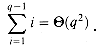

Figure 22.2 (a) Linked-list representations of two sets. One contains objects b, c, e, and h, with c as the representative, and the other contains objects d, f, and g, with f as the representative. Each object on the list contains a set member, a pointer to the next object on the list, and a pointer back to the first object on the list, which is the representative. (b) The result of UNION(e, g). The representative of the resulting set is f.
Figure 22.3 A sequence of m operations that takes O(m2) time using the linked-list set representation and the simple implementation of UNION. For this example, n =
m/2+1 and q = m - n.(n+q2), which is(m2) since n = (m) and q = (m). Thus, on the average, each operation requires (m) time. That is, the amortized time of an operation is (m).A weighted-union heuristic
(m) time per call because we may be appending a longer list onto a shorter list; we must update the pointer to the representative for each member of the longer list. Suppose instead that each representative also includes the length of the list (which is easily maintained) and that we always append the smaller list onto the longer, with ties broken arbitrarily. With this simple weighted-union heuristic, a single UNION operation can still take  (m) time if both sets have (m) members. As the following theorem shows, however, a sequence of m MAKE-SET, UNION, and FIND-SET operations, n of which are MAKE-SET operations, takes O(m + n 1g n) time.
 n, after x's representative pointer has been updated 1g k times, the resulting set must have at least k members. Since the largest set has at most n members, each object's representative pointer has been updated at most 1g n times over all the UNION operations. The total time used in updating the n objects is thus O(n 1g n).
 Exercises
1 for i
 1 to 16
2 do MAKE-SET(xi)
3 for i
1 to 15 by 24 do UNION(xi,xi+1)
5 for i
1 to 13 by 46 do UNION(xi,xi+2)
7 UNION(x1,x5)
8 UNION(x11,x13)
9 UNION (x1,x10)
10 FIND-SET(x2)
11 FIND-SET(x9)
22.3 Disjoint-set forests

Figure 22.4 A disjoint-set forest. (a) Two trees representing the two sets of Figure 22.2. The tree on the left represents the set {b, c, e, h}, with c as the representative, and the tree on the right represents the set {d, f, g}, with f as the representative. (b) The result of UNION(e, g).
Heuristics to improve the running time

Figure 22.5 Path compression during the operation FIND-SET. Arrows and self-loops at roots are omitted. (a) A tree representing a set prior to executing FIND-SET(a). Triangles represent subtrees whose roots are the nodes shown. Each node has a pointer to its parent. (b) The same set after executing FIND-SET (a). Each node on the find path now points directly to the root.
Pseudocode for disjoint-set forests
MAKE-SET(x)
1 p[x]
x2 rank[x]
0UNION(x,y)
1 LINK(FIND-SET(x), FIND-SET(y))
LINK(x,y)
1 if rank[x] > rank[y]
2 then p[y]
x3 else p[x]
y4 if rank[x] = rank[y]
5 then rank[y]
rank[y] + 1FIND-SET(x)
1 if x
p[x]2 then p[x]
FIND-SET(p[x])3 return p[x]
Effect of the heuristics on the running time
(â log(1 + â/n)n) if â n and (n + â lg n) if â < n. (m, n)), where (m, n) is the very slowly growing inverse of Ackermann's function, which we define in Section 22.4. In any conceivable application of a disjoint-set data structure, (m, n) 4; thus, we can view the running time as linear in m in all practical situations. In Section 22.4, we prove the slightly weaker bound of O(m lg* n).
Exercises
(m lg n) time when we use union by rank only.* 22.4 Analysis of union by rank with path compression
(m, n)) for m disjoint-set operations on n elements. In this section, we shall examine the function to see just how slowly it grows. Then, rather than presenting the very complex proof of the O(m (m, n)) running time, we shall offer a simpler proof of a slightly weaker upper bound on the running time: O(m lg* n).Ackermann's function and its inverse
, it helps to have a notation for repeated exponentiation. For an integer i 0, the expression
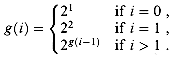
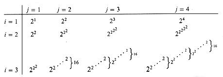
Figure 22.6 Values of A(i, j) for small values of i and j.
 0:
0: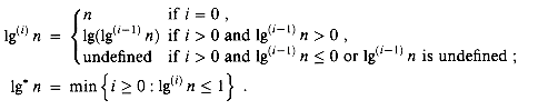
 1 by
1 byA(1,j) = 2j for j
1 ,A(i,1) = A(i - 1,2) for i
2 ,A(i,j) = A(i - 1,A(i,j - 1)) for i,j
2 . , . . . of the first row. Lines between adjacent rows indicate columns in the lower-numbered row that are in the subset included in the higher-numbered row. The third row consists of the even more widely spaced subset of columns
 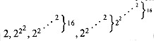 , . . . of the second row, which is an even sparser subset of columns of the first row. In general, the spacing between columns of row i - 1 appearing in row i increases dramatically with both the column number and the row number. Observe that
 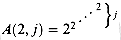 for all integers j 1. Thus, for i > 2, the function A(i, j) grows even more quickly than
  .
.
Figure 22.7 The explosive growth of Ackermann's function. Lines between rows i - 1 and i indicate entries of row i - 1 appearing in row i. Due to the explosive growth, the horizontal spacing is not to scale. The horizontal spacing between entries of row i - 1 appearing in row i greatly increases with the column number and row number. If we trace the entries in row i to their original appearance in row 1, the explosive growth is even more evident.
(m,n) = min {i 1: A(i, m/n) > lg n} .(m, n)) running time, which is beyond the scope of this book.(m, n) is monotonically decreasing. To see this property, note that m/n is monotonically increasing as m increases; therefore, since n is fixed, the smallest value of i needed to bring A(i,m/n) above lg n is monotonically decreasing. This property corresponds to our intuition about disjoint-set forests with path compression: for a given number of distinct elements n, as the number of operations m increases, we would expect the average find-path length to decrease due to path compression. If we perform m operations in time O(m (m, n)), then the average time per operation is O((m, n)), which is monotonically decreasing as m increases.(m, n) 4 for all practical purposes, we first note that the quantity m/n is at least 1, since m n. Since Ackermann's function is strictly increasing with each argument, m/n 1 implies A(i, m/n) A(i, 1) for all i 1. In particular, A(4, m/n) A(4, 1). But we also have that 1g n, and thus (m, n) 4 for all practical purposes. Note that the O(m 1g* n) bound is only slightly weaker than the O(m (m, n)) bound; 1g*65536 = 4 and 1g* 265536 = 5, so 1g* n 5 for all practical purposes.
Properties of ranks
rank[p[x]], with strict inequality if x p[x]. The value of rank[x] is initially 0 and increases through time until x p[x]; from then on, rank[x] does not change. The value of rank[p[x]] is a monotonically increasing function of time. 2rank[x]. rank[y], assume without loss of generality that rank[x] < rank[y]. Node y is the root of the tree formed by the LINK operation, andsize'(y) = size(x) + size(y)
2rank[x] + 2rank[y] 2rank[y]= 2rank'[y].
size'(y) = size(x) + size(y)
2rank[x] + 2rank[y]= 2rank[y]+ 1
= 2rank'[y] .
0, there are at most n/2r nodes of rank r.1g n.Proving the time bound
m 3m'. Since m = O(m'), an O(m 1g* n) time bound for the converted sequence S implies an O(m' 1g* n) time bound for the original sequence S'. 1g n. (Recall that 1g n is the maximum rank.) The highest-numbered block is therefore block 1g*(1g n) = 1g* n - 1. For notational convenience, we define for integers j -1,
{B(j - 1) + 1, B(j - 1) + 2, . . . , B(j)} . xl remains the same, but the new parent of xi has a rank strictly greater than that of xi's old parent. The difference between the ranks of xi and its parent is a monotonically increasing function of time. Thus, the difference between 1g* rank[p[xi]] and 1g* rank[xi] is also a monotonically increasing function of time. Once xi and its parent have ranks in different blocks, they will always have ranks in different blocks, and so xi will never again be assessed a path charge. xl before path compression, so that xi will be assigned a new parent during path compression. Moreover, as we have observed, xi's new parent has a higher rank than its old parent. Suppose that node xi's rank is in block j. How many times can xi be assigned a new parent, and thus assessed a path charge, before xiis assigned a parent whose rank is in a different block (after which xi will never again be assessed a path charge)? This number of times is maximized if xi has the lowest rank in its block, namely B(j - 1) + 1, and its parents' ranks successively take on the values B(j - 1) + 2, B(j - 1) + 3, . . . , B(j). Since there are B(j) - B(j - 1) - 1 such ranks, we conclude that a vertex can be assessed at most B(j) - B(j - 1) - 1 path charges while its rank is in block j. 0. (Recall that by Lemma 22.2, the rank of a node is fixed once it becomes a child of another node.) Let the number of nodes whose ranks are in block j be denoted by N(j). Then, by Lemma 22.4,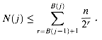
N(0) = n/20 + n/21
= 3n/2
= 3n/2B(0).
1, we have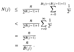 3n/2B(j) for all integers j 0.
 n. Since there are O(n) MAKE-SET and LINK operations, with one charge each, the total time is O(m 1g* n).
 Exercises
(m) path charges could be assessed a given node while its rank is in a given block j.Problems
4, 8, E, 3, E, 9, 2, 6, E, E, E, 1, 7, E, 5.
I1,E,I2,E,I3,...,Im,E,Im+1 ,
OFF-LINE-MINIMUM(m,n)
1 for i
1 to n2 do determine j such that i
Kj3 if j
m + 14 then extracted[j]
i5 let l be the smallest value greater than j
for which set Kl exists
6 Kl
Kj Kl, destroying Kj7 return extracted
v and FIND-DEPTH(v) by following the find path up to the root, returning a count of all nodes other than v encountered, show that the worst-case running time of a sequence of m MAKE-TREE, FIND-DEPTH, and GRAFT operations is (m2).
LCA(u)
1 MAKE-SET(u)
2 ancestor[FIND-SET(u)]
u3 for each child v of u in T
4 do LCA(v)
5 UNION(u,v)
6 ancestor[FIND-SET(u)]
u7 color[u]
BLACK8 for each node v such that {u,v} P9 do if color[v] = BLACK
10 then print "The least common ancestor of"
u "and" v "is" ancestor [FIND-SET(v)]
P. P.Chapter notes
(m,n)) was first given by Tarjan[186, 188]. The O(m 1g* n) upper bound was proven earlier by Hopcroft and Ullman[4, 103]. Tarjan and van Leeuwen [190] discuss variants on the path-compression heuristic, including "one-pass methods," which sometimes offer better constant factors in their performance than do two-pass methods. Gabow and Tarjan [76] show that in certain applications, the disjoint-set operations can be made to run in O(m) time.(m (m, n)) time is required for operations on any disjoint-set data structure satisfying certain technical conditions. This lower bound was later generalized by Fredman and Saks [74], who showed that in the worst case, (m (m, n)) (1g n)-bit words of memory must be accessed.