


In this chapter, we consider the problem of finding shortest paths between all pairs of vertices in a graph. This problem might arise in making a table of distances between all pairs of cities for a road atlas. As in Chapter 25, we are given a weighted, directed graph G = (V, E) with a weight function w: E
We can solve an all-pairs shortest-paths problem by running a single-source shortest-paths algorithm
If negative-weight edges are allowed, Dijkstra's algorithm can no longer be used. Instead, we must run the slower Bellman-Ford algorithm once from each vertex. The resulting running time is O(V2 E), which on a dense graph is O(V4). In this chapter we shall see how to do better. We shall also investigate the relation of the all-pairs shortest-paths problem to matrix multiplication and study its algebraic structure.
Unlike the single-source algorithms, which assume an adjacency-list representation of the graph, most of the algorithms in this chapter use an adjacency-matrix representation. (Johnson's algorithm for sparse graphs uses adjacency lists.) The input is an n
Negative-weight edges are allowed, but we assume for the time being that the input graph contains no negative-weight cycles.
The tabular output of the all-pairs shortest-paths algorithms presented in this chapter is an n
To solve the all-pairs shortest-paths problem on an input adjacency matrix, we need to compute not only the shortest-path weights but also a predecessor matrix
and
If G
In order to highlight the essential features of the all-pairs algorithms in this chapter, we won't cover the creation and properties of predecessor matrices as extensively as we dealt with predecessor subgraphs in Chapter 25. The basics are covered by some of the exercises.
Section 26.1 presents a dynamic-programming algorithm based on matrix multiplication to solve the all-pairs shortest-paths problem. Using the technique of "repeated squaring," this algorithm can be made to run in
Before proceeding, we need to establish some conventions for adjacency-matrix representations. First, we shall generally assume that the input graph G = (V, E) has n vertices, so that n =
This section presents a dynamic-programming algorithm for the all-pairs shortest-paths problem on a directed graph G = (V, E). Each major loop of the dynamic program will invoke an operation that is very similar to matrix multiplication, so that the algorithm will look like repeated matrix multiplication. We shall start by developing a
Before proceeding, let us briefly recap the steps given in Chapter 16 for developing a dynamic-programming algorithm.
1. Characterize the structure of an optimal solution.
2. Recursively define the value of an optimal solution.
3. Compute the value of an optimal solution in a bottom-up fashion.
(The fourth step, constructing an optimal solution from computed information, is dealt with in the exercises.)
We start by characterizing the structure of an optimal solution. For the all-pairs shortest-paths problem on a graph G = (V, E), we have proved (Lemma 25.1 ) that all subpaths of a shortest path are shortest paths.Supppose that the graph is represented by an adjacency matrix W = (wij). Consider a shortest path p from vertex i to vertex j, and suppose that p containsat most m edges. Assuming that there are no negative-weight cycles, m is finite. If i = j, then p has weight 0 and no edges. If vertices i and j are distinct, then we decompose path p into
Now, let
For m
The latter equality follows since wjj = 0 for all j.
What are the actual shortest-path weights
Taking as our in put the matrix W = (wij), we now compute a series of matrices D(1), D(2), . . . , D(n-1), where for m = 1, 2, . . . n - 1,, we have
The heart of the algorithm is the following procedure, which, given matrices D(m-1) and W, returns the matrix D(m). That is, it extends the shortest paths computed so far by one more edge.
The procedure computes a matrix D' = (d'ij), which it returns at the end. It does so by computing equation (26.2) for all i and j, using D for D(m-1)and D' for D(m). (It is written without the superscripts to make its input and output matrices independent of m.) Its running time is
We can now see the relation to matrix multiplication. Suppose we wish to compute the matrix product C = A
Observe that if we make the substitutions
in equation (26.2), we obtain equation (26.4). Thus, if we make these changes to EXTEND-SHORTEST-PATHS and also replace
Returning to the all-pairs shortest-paths problem, we compute the shortest-path weights by extending shortest paths edge by edge. Letting A
As we argued above, the matrix D(n-1) = Wn-1 contains the shortest-path weights. The following procedure computes this sequence in
Figure 26.1 shows a graph and the matrices D(m) computed by the procedure SLOW-ALL-PAIRS-SHORTEST-PATHS.
Our goal, however, is not to compute all the D(m) matrices: we are interested only in matrix D(n-1). Recall that in the absence of negative-weight cycles, equation (26.3) implies D(m) = D(n-1) for all integers m
Since 2
The following procedure computes the above sequence of matrices by using this technique of repeated squaring.
In each iteration of the while loop of lines 4-6, we compute D(2m) = (D(m))2, starting with m = 1. At the end of each iteration, we double the value of m. The final iteration computes D(n-1) by actually computing D(2m) for some n - 1
The running time of FASTER-ALL-PAIRS-SHORTEST-PATHS is
26.1-1
Run SLOW-ALL-PAIRS-SHORTEST-PATHS on the weighted, directed graph of Figure 26.2, showing the matrices that result for each iteration of the respective loops. Then do the same for FASTER-ALL-PAIRS-SHORTEST-PATHS.
26.1-2
Why do we require that wii = 0 for all 1
26.1-3
What does the matrix
used in the shortest-paths algorithms correspond to in regular matrix multiplication?
26.1-4
Show how to express the single-source shortest-paths problem as a product of matrices and a vector. Describe how evaluating this product corresponds to a Bellman-Ford-like algorithm (see Section 25.3).
26.1-5
Suppose we also wish to compute the vertices on shortest paths in the algorithms of this section. Show how to compute the predecessor matrix
26.1-6
The vertices on shortest paths can also be computed at the same time as the shortest-path weights. Let us define
26.1-7
The FASTER-ALL-PAIRS-SHORTEST-PATHS procedure, as written, requires us to store
26.1-8
Modify FASTER-ALL-PAIRS-SHORTEST-PATHS to detect the presence of a negative-weight cycle.
26.1-9
Give an efficient algorithm to find the length (number of edges) of a minimum-length negative-weight cycle in a graph.
In this section, we shall use a different dynamic-programming formulation to solve the all-pairs shortest-paths problem on a directed graph G = (V, E). The resulting algorithm, known as the Floyd-Warshall algorithm, runs in
In the Floyd-Warshall algorithm, we use a different characterization of the structure of a shortest path than we used in the matrix-multiplication-based all-pairs algorithms. The algorithm considers the "intermediate" vertices of a shortest path, where an intermediate vertex of a simple path p =
The Floyd-Warshall algorithm is based on the following observation. Let the vertices of G be V = {1, 2, . . . , n}, and consider a subset {1, 2, . . . , k} of vertices for some k. For any pair of vertices i, j
Based on the above observations, we define a different recursive formulation of shortest-path estimates than we did in Section 26.1. Let
The matrix
Based on recurrence (26.5), the following bottom-up procedure can be used to compute the values
Figure 26.4 shows a directed graph and the matrices D(k) computed by the Floyd-Warshall algorithm.
The running time of the Floyd-Warshall algorithm is determined by the triply nested for loops of lines 3-6. Each execution of line 6 takes O(1) time. The algorithm thus runs in time
There are a variety of different methods for constructing shortest paths in the Floyd-Warshall algorithm. One way is to compute the matrix D of shortest-path weights and then construct the predecessor matrix
We can compute the predecessor matrix
We can give a recursive formulation of
For k
We leave the incorporation of the
Given a directed graph G = (V, E) with vertex set V = {1, 2, . . . , n}, we may wish to find out whether there is a path in G from i to j for all vertex pairs i, j
E* = {(i, j) : there is a path from vertex i to vertex j in G} .
One way to compute the transitive closure of a graph in
There is another, similar way to compute the transitive closure of G in
and for k
As in the Floyd-Warshall algorithm, we compute the matrices
Figure 26.5 shows the matrices T(k) computed by the TRANSITIVE-CLOSURE procedure on a sample graph. Like the Floyd-Warshall algorithm, the running time of the TRANSITIVE-CLOSURE procedure is
In Section 26.4, we shall see that the correspondence between FLOYD-WARSHALL and TRANSITIVE-CLOSURE is more than coincidence. Both algorithms are based on a type of algebraic structure called a "closed semiring."
26.2-1
Run the Floyd-Warshall algorithm on the weighted, directed graph of Figure 26.2. Show the matrix D(k) that results for each iteration of the outer loop.
26.2-2
As it appears above, the Floyd-Warshall algorithm requires
26.2-3
Modify the FLOYD-WARSHALL procedure to include computation of the
26.2-4
Suppose that we modify the way in which equality is handled in equation (26.7):
Is this alternative definition of the predecessor matrix
26.2-5
How can the output of the Floyd-Warshall algorithm be used to detect the presence of a negative-weight cycle?
26.2-6
Another way to reconstruct shortest paths in the Floyd-Warshall algorithm uses values
26.2-7
Give an O(V E)-time algorithm for computing the transitive closure of a directed graph G = (V, E).
26.2-8
Suppose that the transitive closure of a directed acyclic graph can be computed in
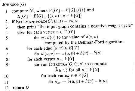
Johnson's algorithm finds shortest paths between all pairs in O(V2 lg V + V E) time; it is thus asymptotically better than either repeated squaring of matrices or the Floyd-Warshall algorithm for sparse graphs. The algorithm either returns a matrix of shortest-path weights for all pairs or reports that the input graph contains a negative-weight cycle. Johnson's algorithm uses as subroutines both Dijkstra's algorithm and the Bellman-Ford algorithm, which are described in Chapter 25.
Johnson's algorithm uses the technique of reweighting, which works as follows. If all edge weights w in a graph G = (V, E) are nonnegative, we can find shortest paths between all pairs of vertices by running Dijkstra's algorithm once from each vertex; with the Fibonacci-heap priority queue, the running time of this all-pairs algorithm is O(V2 lg V + V E). If G has negative-weight edges, we simply compute a new set of nonnegative edge weights that allows us to use the same method. The new set of edge weights
1. For all pairs of vertices u, v
2. For all edges (u, v), the new weight
As we shall see in a moment, the preprocessing of G to determine the new weight function
As the following lemma shows, it is easy to come up with a reweighting of the edges that satisfies the first property above. We use
Lemma 26.1
Given a weighted, directed graph G = (V, E) with weight function w: E
Let p =
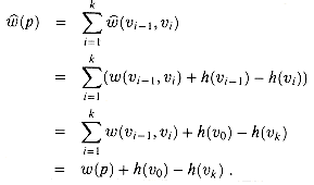
Proof We start by showing that
We have
The third equality follows from the telescoping sum on the second line.
We now show by contradiction that w(p) =
which implies that w(p') < w(p). But this contradicts our assumption that p is a shortest path from u to v using w. The proof of the converse is similar.
Finally, we show that G has a negative-weight cycle using weight function w if and only if G has a negative-weight cycle using weight function
and thus c has negative weight using w if and only if it has negative weight using
Our next goal is to ensure that the second property holds: we want
Now suppose that G and G' have no negative-weight cycles. Let us define h(v) =
Johnson's algorithm to compute all-pairs shortest paths uses the Bellman-Ford algorithm (Section 25.3) and Dijkstra's algorithm (Section 25.2) as subroutines. It assumes that the edges are stored in adjacency lists. The algorithm returns the usual
This code simply performs the actions we specified earlier. Line 1 produces G'. Line 2 runs the Bellman-Ford algorithm on G' with weight function w. If G' , and hence G, contains a negative-weight cycle, line 3 reports the problem. Lines 4-11 assume that G' contains no negative-weight cycles. Lines 4-5 set h(v) to the shortest-path weight
The running time of Johnson's algorithm is easily seen to be O(V2 lg V + VE) if the priority queue in Dijkstra's algorithm is implemented by a Fibonacci heap. The simpler binary-heap implementation yields a running time of O(V E 1g V), which is still asymptotically faster than the Floyd-Warshall algorithm if the graph is sparse.
26.3-1
Use Johnson's algorithm to find the shortest paths between all pairs of vertices in the graph of Figure 26.2. Show the values of h and
26.3-2
What is the purpose of adding the new vertex s to V, yielding V'?
26.3-3
Suppose that w(u, v)
In this section, we examine "closed semirings," an algebraic structure that yields a general framework for solving path problems in directed graphs. We start by defining closed semirings and discussing how they relate to a calculus of directed paths. We then show some examples of closed semirings and a "generic" algorithm for computing all-pairs path information. Both the Floyd-Warshall algorithm and the transitive-closure algorithm from Section 26.2 are instantiations of this generic algorithm.
A closed semiring is a system
1.
Likewise,
3.
4.
6. If a1, a2, a3, . . . is a countable sequence of elements of S, then a1
7. Associativity, commutativity, and idempotence apply to infinite summaries. (Thus, any infinite summary can be rewritten as an infinite summary in which each term of the summary is included just once and the order of evaluation is arbitrary.)
Although the closed-semiring properties may seem abstract, they can be related to a calculus of paths in directed graphs. Suppose we are given a directed graph G = (V, E) and a labeling function
We use the associative extension operator
The identity
As a runing example of an application of closed semirings, we shall use shortest paths with nonnegative edge weights. The codomain S is R
Not surprisingly, the role of
Because the extension operator
and the label of their concatenation is
The summary operator
Our goal will be to compute, for all pairs of vertices i, j
We require commutativity and associativity of
For shortest paths, we use min as the summary operator
We want the summary operator
Because we consider paths that may not be simple, there may be a countably infinite number of paths in a graph. (Each path, simple or not, has a finite number of edges.) The operator
Returning to the shortest-paths example, we ask if min is applicable to an infinite sequence of values in R
To compute labels of diverging paths, we need distributivity of the extension operator
Because there may be a countably infinite number of paths in a graph,
We use a special notation to denote the label of a cycle that may be traversed any number of times. Suppose that we have a cycle c with label
Thus, in Figure 26.8, we want to compute
For the shortest-paths example, for any nonnegative real a
The interpretation of this property is that since all cycles have nonnegative weight, no shortest path ever needs to traverse an entire cycle.
We have already seen one example of a closed semiring, namely S1 = (R
We claimed, however, that even if there are negative-weight edges, the Floyd-Warshall algorithm computes shortest-path weights as long as no negative-weight cycles are present. By adding the appropriate closure operator and extending the codomain of labels to R
The second case (a < 0) models the situation in which we can traverse a negative-weight cycle an infinite number of times to obtain a weight of -
For transitive closure, we use the closed semiring S3 = ({0, 1}, V,
Suppose we are given a directed graph G = (V, E) with labeling function
which is the result of summarizing all paths from i to j using the summary operator
There is a dynamic-programming algorithm to solve this problem, and its form is very similar to the Floyd-Warshall algorithm and the transitive- closure algorithm. Let
Note the analogy to the definitions of
Recurrence (26.12) is reminiscent of recurrences (26.5) and (26.8), but with an additional factor of
which we can see as follows. The label of the one-edge path <i, j> is simply
The dynamic-programming algorithm computes the values
The running time of this algorithm depends on the time to compute
26.4-1
Verify that S1 = (R
26.4-2
Verify that S2 = (R
26.4-3
Rewrite the COMPUTE-SUMMARIES procedure to use closed semiring S2, so that it implements the Floyd-Warshall algorithm. What should be the value of -
26.4-4
Is the system S4 = (R, +,
26.4-5
Can we use an arbitrary closed semiring for Dijkstra's algorithm? What about for the Bellman-Ford algorithm? What about for the FASTER-ALL-PAIRS-SHORTEST-PATHS procedure?
26.4-6
A trucking firm wishes to send a truck from Castroville to Boston laden as heavily as possible with artichokes, but each road in the United States has a maximum weight limit on trucks that use the road. Model this problem with a directed graph G = (V, E) and an appropriate closed semiring, and give an efficient algorithm to solve it.
26-1 Transitive closure of a dynamic graph
Suppose that we wish to maintain the transitive closure of a directed graph G = (V, E) as we insert edges into E. That is, after each edge has been inserted, we want to update the transitive closure of the edges inserted so far. Assume that the graph G has no edges initially and that the transitive closure is to be represented as a boolean matrix.
a. Show how the transitive closure G* = (V, E*) of a graph G = (V, E) can be updated in 0(V2) time when a new edge is added to G.
b. Give an example of a graph G and an edge e such that
c. Describe an efficient algorithm for updating the transitive closure as edges are inserted into the graph. For any sequence of n insertions, your algorithm should run in total time
26-2 Shortest paths in
A graph G = (V, E) is
a. What are the asymptotic running times for INSERT, EXTRACT-MIN, and DECREASE-KEY, as a function of d and the number n of elements in a d-ary heap? What are these running times if we choose d =
b. Show how to compute shortest paths from a single source on an
c. Show how to solve the all-pairs shortest-paths problem on an
d. Show how to solve the all-pairs shortest-paths problem in O(V E) time on an
26-3 Minimum spanning tree as a closed semiring
Let G = (V, E) be a connected, undirected graph with weight function w : E
a. Briefly justify the assertion that S = (R
Since S is a closed semiring, we can use the COMPUTE-SUMMARIES procedure to determine the minimax weights mij in graph G. Let
b. Give a recurrence for
c. Let Tm = {(i, j)
d. Show that Tm = T. (Hint: Consider the effect of adding edge (i, j) to T and removing an edge on another path from i to j. Consider also the effect of removing edge (i, j) from T and replacing it with another edge.)
Lawler [132] has a good discussion of the all-pairs shortest-paths problem, although he does not analyze solutions for sparse graphs. He attributes the matrix-multiplication algorithm to the folklore. The Floyd-Warshall algorithm is due to Floyd [68], who based it on a theorem of Warshall [198] that describes how to compute the transitive closure of boolean matrices. The closed-semiring algebraic structure appears in Aho, Hopcroft, and Ullman [4]. Johnson's algorithm is taken from [114].
 R that maps edges to real-valued weights. We wish to find, for every pair of vertices u, v
  V, a shortest (least-weight) path from u to v, where the weight of a path is the sum of the weights of its constituent edges. We typically want the output in tabular form: the entry in u's row and v's column should be the weight of a shortest path from u to v.
 V times, once for each vertex as the source. If all edge weights are nonnegative, we can use Dijkstra's algorithm. If we use the linear-array implementation of the priority queue, the running time is O(V3 + VE) = O(V3). The binary-heap implementation of the priority queue yields a running time of O(V E lg V), which is an improvement if the graph is sparse. Alternatively, we can implement the priority queue with a Fibonacci heap, yielding a running time of O(V2 lg V + VE).
 n matrix W representing the edge weights of an n-vertex directed graph G = (V, E). That is, W = (wij), where
(26.1)
n matrix D = (dij), where entry dij contains the weight of a shortest path from vertex i to vertex j. That is, if we let  (i,j) denote the shortest-path weight from vertex i to vertex j (as in Chapter 25), then dij = (i,j) at termination.
 = (ij ), where ij is NIL if either i = j or there is no path from i to j, and otherwise ij is some predecessor of j on a shortest path from i. Just as the predecessor subgraph G from Chapter 25 is a shortest-paths tree for a given source vertex, the subgraph induced by the ith row of the matrix should be a shortest-paths tree with root i. For each vertex i V, we define the predecessor subgraph of G for i as G,i = (V,i, E,i), where
V
,i = {j V : ij  NIL}
NIL}  {i}
{i}E
,i = {(ij, j): j V,i and ij NIL} .,i is a shortest-paths tree, then the following procedure, which is a modified version of the PRINT-PATH procedure from Chapter 23, prints a shortest path from vertex i to vertex j.PRINT-ALL-PAIRS-SHORTEST-PATH(
,i,j)1 if i = j
2 then print i
3 else if
ij = NIL4 then print "no path from" i "to" j "exists"
5 else PRINT-ALL-PAIRS-SHORTEST-PATH(
,i,ij)6 print j
Chapter outline
 (V3 1g V) time. Another dynamic-programming algorithm, the Floyd-Warshall algorithm, is given in Section 26.2. The Floyd-Warshall algorithm runs in time (V3). Section 26.2 also covers the problem of finding the transitive closure of a directed graph, which is related to the all-pairs shortest-paths problem. Johnson's algorithm is presented in Section 26.3. Unlike the other algorithms in this chapter, Johnson's algorithm uses the adjacency-list representation of a graph. It solves the all-pairs shortest-paths problem in O(V2 lg V + V E) time, which makes it a good algorithm for large, sparse graphs. Finally, in Section 26.4, we examine an algebraic structure called a "closed semiring," which allows many shortest-paths algorithms to be applied to a host of other all-pairs problems not involving shortest paths.V. Second, we shall use the convention of denoting matrices by uppercase letters, such as W or D, and their individual elements by subscripted lowercase letters, such as wij or dij. Some matrices will have parenthesized superscripts, as in D(m) =
  , to indicate iterates. Finally, for a given n n matrix A, we shall assume that the value of n is stored in the attribute rows[A].
26.1 Shortest paths and matrix multiplication
(V4)-time algorithm for the all-pairs shortest-paths problem and then improve its running time to (V3 lg V).The structure of a shortest path
 , where path p' now contains at most m - 1 edges. Moreover, by Lemma 25.1, p' is a shortest path from i to k. Thus, by Corollary 25.2, we have (i, j) = (i, k) + wkj.
A recursive solution to the all-pairs shortest-paths problem
 be the minimum weight of any path from vertex i to vertex j that contains at most m edges. When m = 0, there is a shortest path from i to j with no edges if and only if i = j. Thus,
 1, we compute
  as the minimum of
  (the weight of the shortest path from i to j consisting of at most m - 1 edges) and the minimum weight of any path from i to j consisting of at most m edges, obtained by looking at all possible predecessors k of j. Thus, we recursively define
(26.2)
(i, j)? If the graph contains no negative-weight cycles, then all shortest paths are simple and thus contain at most n - 1 edges. A path from vertex i to vertex j with more than n - 1 edges cannot have less weight than a shortest path from i to j. The actual shortest-path weights are therefore given by
(26.3)
Computing the shortest-path weights bottom up
 . The final matrix D(n-1) contains the actual shortest-path weights. Observe that since
  for all vertices i, j V, we have D(1) = W.
EXTEND-SHORTEST-PATHS(D,W)
1 n
 rows[D]
2 let D' = (d'ij) be an n
n matrix3 for i
1 to n4 do for j
1 to n5 do d'ij

6 for k
1 to n7 do d'ij
min(d'ij, dik + wkj)8 return D'
(n3) due to the three nested for loops. B of two n n matrices A and B. Then, for i, j = 1, 2, . . . , n, we compute
(26.4)
d(m-1)
a ,w
b ,d(m)
c ,min
+ ,+
(the identity for min) by 0 (the identity for +), we obtain the straightforward (n3)-time procedure for matrix multiplication.MATRIX-MULTIPLY(A, B)
1 n
rows[A]2 let C be an n
n matrix3 for i
1 to n4 do for j
1 to n5 do cij
06 for k
1 to n7 do cij
cij + aik bkj8 return C
B denote the matrix "product" returned by EXTEND-SHORTEST-PATHS(A, B), we compute the sequence of n - 1 matricesD(1) = D(0)
W = W,D(2) = D(1)
W = W2,D(3) = D(2)
W = W3,
D(n-1) = D(n-2)
W = Wn-1 .(n4) time.SLOW-ALL-PAIRS-SHORTEST-PATHS(W)
1 n
rows[W]2 D(1)
W3 for m
2 to n - 14 do D(m)
EXTEND-SHORTEST-PATHS(D(m-1),W)5 return D(n-1)
Improving the running time
n - 1. We can compute D(n-1) with only  lg(n - 1)
 matrix products by computing the sequence
D(1) = W ,
D(2) = W2 = W
W,D(4) = W4 = W2
W2D(8) = W8 = W4
W4,
D(2
lg(n-1)) = W2lg(n-1) = W2lg(n-1)-1 W2lg(n-1)-1.lg(n-1) n - 1, the final product D(21g(n-1)) is equal to D(n-1).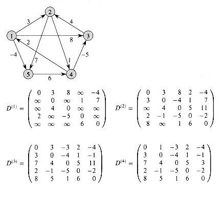
Figure 26.1 A directed graph and the sequence of matrices D(m) computed by SLOW-ALL-PAIRS-SHORTEST-PATHS. The reader may verify that D(5) = D(4) . W is equal to D(4), and thus D(m) = D(4) for all m
4.FASTER-ALL-PAIRS-SHORTEST-PATHS(W)
1 n
rows[W]2 D(1)
W3 m
14 while n - 1 > m
5 do D(2m)
EXTEND-SHORTEST-PATHS(D(m),D(m))6 m
2m7 return D(m)
 2m < 2n - 2. By equation (26.3), D(2m) = D(n-1). The next time the test in line 4 is performed, m has been doubled, so now n - 1 m, the test fails, and the procedure returns the last matrix it computed.(n3lg n) since each of the lg(n - 1) matrix products takes (n3) time. Observe that the code is tight, containing no elaborate data structures, and the constant hidden in the -notation is therefore small.
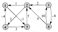
Figure 26.2 A weighted, directed graph for use in Exercises 26.1-1, 26.2-1, and 26.3-1.
Exercises
i n?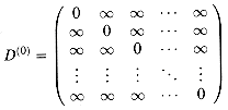 from the completed matrix D of shortest-path weights in O(n3) time.
 to be the predecessor of vertex j on any minimum-weight path from i to j that contains at most m edges. Modify EXTEND-SHORTEST-PATHS and SLOW-ALL-PAIRS-SHORTEST-PATHS to compute the matrices (1), (2), . . . , (n-1) as the matrices D(1), D(2), . . . , D(n-1) are computed.lg(n - 1) matrices, each with n2 elements, for a total space requirement of (n2 lg n). Modify the procedure to require only (n2) space by using only two n n matrices.
26.2 The Floyd-Warshall algorithm
(V3) time. As before, negative-weight edges may be present, but we shall assume that there are no negative-weight cycles. As in Section 26.1, we shall follow the dynamic-programming process to develop the algorithm. After studying the resulting algorithm, we shall present a similar method for finding the transitive closure of a directed graph.The structure of a shortest path
 v1, v2, . . . , vl
 is any vertex of p other than v1 or vl, that is, any vertex in the set {v2,v3, . . . , vl-1}. V, consider all paths from i to j whose intermediate vertices are all drawn from {1, 2, . . . , k}, and let p be a minimum-weight path from among them. (Path p is simple, since we assume that G contains no negative-weight cycles.) The Floyd- Warshall algorithm exploits a relationship between path p and shortest paths from i to j with all intermediate vertices in the set {1, 2, . . . , k - 1}. The relationship depends on whether or not k is an intermediate vertex of path p.
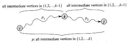
Figure 26.3 Path p is a shortest path from vertex i to vertex j, and k is the highest-numbered intermediate vertex of p. Path p1, the portion of path p from vertex i to vertex k, has all intermediate vertices in the set {1, 2, . . . , k - 1}. The same holds for path p2 from vertex k to vertex j.
 If k is not an intermediate vertex of path p, then all intermediate vertices of path p are in the set {1, 2, . . . , k - 1}. Thus, a shortest path from vertex i to vertex j with all intermediate vertices in the set {1, 2, . . . , k - 1} is also a shortest path from i to j with all intermediate vertices in the set {1, 2, . . . , k}. If k is an intermediate vertex of path p, then we break p down into
  as shown in Figure 26.3. By Lemma 25.1, p1 is a shortest path from i to k with all intermediate vertices in the set {1, 2, . . . , k}. In fact, vertex k is not an intermediate vertex of path p1, and so p1 is a shortest path from i to k with all intermediate vertices in the set {1, 2, . . . , k - 1}. Similarly, p2 is a shortest path from vertex k to vertex j with all intermediate vertices in the set {1, 2, . . . , k - 1}.
A recursive solution to the all-pairs shortest-paths problem
 be the weight of a shortest path from vertex i to vertex j with all intermediate vertices in the set {1, 2, . . . , k}. When k = 0, a path from vertex i to vertex j with no intermediate vertex numbered higher than 0 has no intermediate vertices at all. It thus has at most one edge, and hence
  . A recursive definition is given by
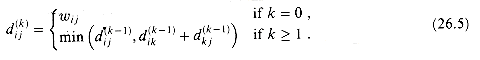
(26.5)
 gives the final answer--
 for all i, j V--because all intermediate vertices are in the set {1, 2, . . . , n}.
Computing the shortest-path weights bottom up
 in order of increasing values of k. Its input is an n n matrix W defined as in equation (26.1). The procedure returns the matrix D(n) of shortest-path weights.
 (n3). As in the final algorithm in Section 26.1, the code is tight, with no elaborate data structures, and so the constant hidden in the -notation is small. Thus, the Floyd-Warshall algorithm is quite practical for even moderate-sized input graphs.
Constructing a shortest path
from the D matrix. This method can be implemented to run in O(n3) time (Exercise 26.1-5). Given the predecessor matrix , the PRINT-ALL-PAIRS-SHORTEST-PATH procedure can be used to print the vertices on a given shortest path. "on-line" just as the Floyd-Warshall algorithm computes the matrices D(k). Specifically, we compute a sequence of matrices (0), (1), . . . , (n), where = (n) and  is defined to be the predecessor of vertex j on a shortest path from vertex i with all intermediate vertices in the set {1, 2, . . . , k}.
 . When k = 0, a shortest path from i to j has no intermediate vertices at all. Thus,
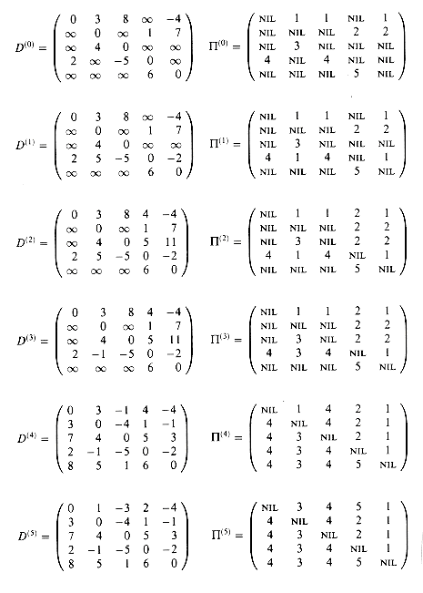
Figure 26.4 The sequence of matrices D(k) and
(k) computed by the Floyd-Warshall algorithm for the graph in Figure 26.1.
(26.6)
1, if we take the path  , then the predecessor of j we choose is the same as the predecessor of j we chose on a shortest path from k with all intermediate vertices in the set {1, 2, . . . , k - 1}. Otherwise, we choose the same predecessor of j that we chose on a shortest path from i with all intermediate vertices in the set {1, 2, . . . , k - 1}. Formally, for k 1,
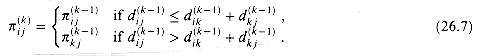
(26.7)
(k) matrix computations into the FLOYD-WARSHALL procedure as Exercise 26.2-3. Figure 26.4 shows the sequence of (k) matrices that the resulting algorithm computes for the graph of Figure 26.1. The exercise also asks for the more difficult task of proving that the predecessor subgraph G,i is a shortest-paths tree with root i. Yet another way to reconstruct shortest paths is given as Exercise 26.2-6.Transitive closure of a directed graph
V. The transitive closure of G is defined as the graph G* = (V, E*), where(n3) time is to assign a weight to 1 to each edge of E and run the Floyd-Warshall algorithm. If there is a path from vertex i to vertex j, we get dij < n. Otherwise, we get dij = .(n3) time that can save time and space in practice. This method involves substitutions of the logical operations  and
and  for the arithmetic operations min and + in the Floyd-Warshall algorithm. For i, j, k = 1, 2, . . . , n, we define
  to be 1 if there exists a path in graph G from vertex i to j with all intermediate vertices in the set {1, 2, . . . , k}, and 0 otherwise. We construct the transitive closure G* = (V, E*) by putting edge (i, j) into E* if and only if
  = 1. A recursive definition of
  , analogous to recurrence (26.5), is
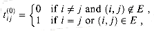 1,
1,
(26.8)
 in order of increasing k.
TRANSITIVE-CLOSURE(G)
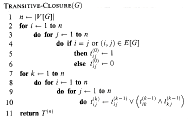 (n3). On some computers, though, logical operations on single-bit values execute faster than arithmetic operations on integer words of data. Moreover, because the direct transitive-closure algorithm uses only boolean values rather than integer values, its space requirement is less than the Floyd-Warshall algorithm's by a factor corresponding to the size of a word of computer storage.
Exercises
(n3) space, since we compute  for i, j, k = 1, 2, . . . , n. Show that the following procedure, which simply drops all the superscripts, is correct, and thus only (n2) space is required.
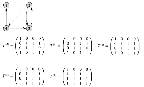
Figure 26.5 A directed graph and the matrices T(k) computed by the transitive-closure algorithm.
FLOYD-WARSHALL'(W)
1 n
rows[W]2 D
W3 for k
1 to n4 do for i
1 to n5 do for j
1 to n6 dij
min(dij, dik + dkj)7 return D
(k) matrices according to equations (26.6) and (26.7). Prove rigorously that for all i V, the predecessor subgraph G, i is a shortest-paths tree with root i. (Hint: To show that G,i is acyclic, first show that  implies
 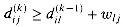 . Then, adapt the proof of Lemma 25.8.)
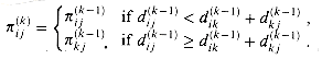 correct?
 for i, j, k = 1, 2, . . . , n, where
  is the highest-numbered intermediate vertex of a shortest path from i to j. Give a recursive formulation for
  , modify the FLOYD-WARSHALL procedure to compute the
  values, and rewrite the PRINT-ALL-PAIRS-SHORTEST-PATH procedure to take the matrix
  as an input. How is the matrix
  like the s table in the matrix-chain multiplication problem of Section 16.1?
 (V, E) time, where (V, E) =
  (V + E) and is monotonically increasing. Show that the time to compute the transitive closure of a general directed graph is O((V, E)).
26.3 Johnson's algorithm for sparse graphs
 must satisfy two important properties. V, a shortest path from u to v using weight function w is also a shortest path from u to v using weight function
  .
. is nonnegative.
 can be performed in O(V E) time.
Preserving shortest paths by reweighting
to denote shortest-path weights derived from weight function w and  to denote shortest-path weights derived from weight function
  . R, let h: V R be any function mapping vertices to real numbers. For each edge (u, v) E, define
(26.9)
v0, vl, . . . , vk) be a path from vertex  0 to vertex vk. Then, w(p) = (v0, vk) if and only if
 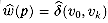 . Also, G has a negative-weight cycle using weight function w if and only if G has a negative-weight cycle using weight function
  .
.
(26.10)
 (v0, vk) implies
 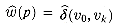 . Suppose that there is a shorter path p' from v0 to vk using weight function
  . Then,
  . By equation (26.10),
 . Consider any cycle c = <v0, v1, . . . , vk>, where v0= vk. By equation (26.10),
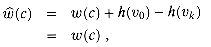

Producing nonnegative weights by reweighting
 (u, v) to be nonnegative for all edges (u,v) E. Given a weighted, directed graph G = (V, E) with weight function : E R, we make a new graph G' = (V', E'), where V' = V {s} for some new vertex s
  V and E'= E {(s, ): v V}. We extend the weight function w so that (s,v) = 0 for all v V. Note that because s has no edges that enter it, no shortest paths in G', other than those with source s, contain s. Moreover, G' has no negative-weight cycles if and only if G has no negative-weight cycles. Figure 26.6(a) shows the graph G' corresponding to the graph G of Figure 26.1.(s,v) for all v V'. By Lemma 25.3, we have h(v) h(u) + (u, v) for all edges (u,v) E'. Thus, if we define the new weights
  according to equation (26.9), we have
  and the second property is satisfied. Figure 26.6(b) shows the graph G' from Figure 26.6(a) with reweighted edges.
Computing all-pairs shortest paths
VXV matrix D = dij, where dij = (i, j), or it reports that the input graph contains a negative-weight cycle. (In order for the indices into the D matrix to make any sense, we assume that the vertices are numbered from 1 to V.)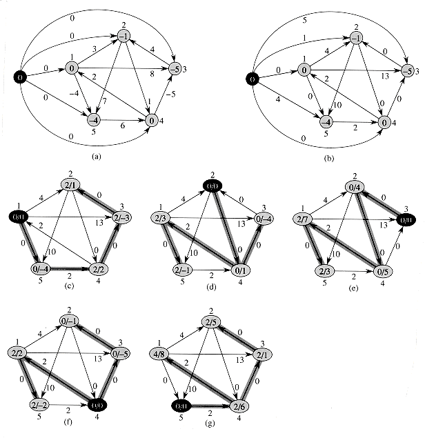
Figure 26.6 Johnson's all-pairs shortest-paths algorithm run on the graph of Figure 26.1. (a) The graph G' with the original weight function w. The new vertex s is black. Within each vertex v is h(v) =
(s, v). (b) Each edge (u, v) is reweighted with weight function  . (c)-(g) The result of running Dijkstra's algorithm on each vertex of G using weight function
  . In each part, the source vertex u is black. Within each vertex v are the values
  and (u, v), separated by a slash. The value duv = (u, v) is equal to
 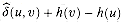 .
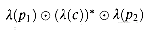
. (s, v) computed by the Bellman-Ford algorithm for all v V'. Lines 6-7 compute the new weights
  . For each pair of vertices u, v V, the for loop of lines 8-11 computes the shortest-path weight
  by calling Dijkstra's algorithm once from each vertex in V. Line 11 stores in matrix entry duv the correct shortest-path weight (u, v), calculated using equation (26.10). Finally, line 12 returns the completed D matrix. Figure 26.6 shows the execution of Johnson's algorithm.
Exercises
 computed by the algorithm. 0 for all edges (u, v) E. What is the relationship between the weight functions w and
  ?
?* 26.4 A general framework for solving path problems in directed graphs
Definition of closed semirings
 where S is a set of elements,
  (the summary operator) and
  (the extension operator) are binary operations on S, and
  are elements of S, satisfying the following eight properties:
 is a monoid: S is closed under : a b S for all a, b S. is associative: a (b c) = (a b) c for all a,b,c S.
 is a monoid.
 is commutative: a b = b a for all a, b S. is idempotent: a a = a for all a S.
 a2 a3 . . . is well defined and in S.
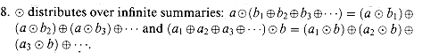
A calculus of paths in directed graphs
 : V X V S mapping all ordered pairs of vertices into some codomain S.The label of edge (u, v) E is denoted ,(u, v). Since is defined over the domain V X V, the label (u, v) is usually taken as
  if (u, v) is not an edge of G (we shall see why in a moment).
 to extend the notion of labels to paths. The label of path p = v1, v2, . . . ,vk is
 serves as the label of the empty path.0 {}, where R0 is the set of nonnegative reals, and (i, j) = wij for all i, j V. The extension operator
  corresponds to the arithmetic operator +, and the label of path p =v1,v2, . . . ,vk is therefore
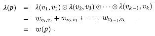
 , the identity for
  , is taken by 0, the identity for +. We denote the empty path by
  , and its label is
 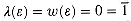 .
. is associative, we can define the label of the concatenation of two paths in a natural way. Given paths p1 = v1,v2, . . . ,vk and p2 = vk,vk+, . . . ,,v1, their concatenation is
p1
 p2 = v1, v2, . . . ,vk,vk+1, . . . ,vl,
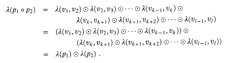 , which is both commutative and associative, is used to summarize path labels. That is, the value (p1) (p2) gives a summary, the semantics of which are specific to the application, of the labels of paths p1 and p2. V, the summary of all path labels from i to j:
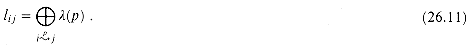
(26.11)
because the order in which paths are summarized should not matter. Because we use the annihilator  as the label of an ordered pair (u, v) that is not an edge in the graph, any path that attempts to take an absent edge has label
  .. The identity for min is , and is indeed an annihilator for + : a + = + a = for all a R0 {}. Absent edges have weight , and if any edge of a path has weight , so does the path. to be idempotent, because from equation (26.11), we see that should summarize the labels of a set of paths. If p is a path, then {p} {p} = {p}; if we summarize path p with itself, the resulting label should be the label of p: (p) (p) = (p). should therefore be applicable to a countably infinite number of path labels. That is, if a1, a2, a3, . . . is a countable sequence of elements in codomain S, then the label a1 a2 a3 . . . should be well defined and in S. It should not matter in which order we summarize path labels, and thus associativity and commutativity should hold for infinite summaries. Furthermore, if we summarize the same path label a a countably infinite number of times, we should get a as the result, and thus idempotence should hold for infinite summaries.0 {}. For example, is the value of min
  well defined? It is, if we think of the min operator as actually returning the greatest lower bound (infimum) of its arguments, in which case we get min
  .
. over the summary operator . As shown in Figure 26.7, suppose that we have paths
  By distributivity, we can summarize the labels of paths p1 2 and p1 3 by computing either
  .
. should distribute over infinite summaries as well as finite ones. Figure 26.8, for example, contains paths
  along with the cycle
  . We must be able to summarize the paths p1 p2, p1 c p2, p1 c c p2, . . . . Distributivity of
  over countably infinite summaries gives us
Figure 26.7 Using distributivity of
 . To summarize the labels of paths p1 p2 and p1 p3, we may compute either
  or
or  .
.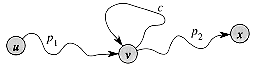
Figure 26.8 Distributivity of
 over countably infinite summaries of . Because of cycle c, there are a countably infinite number of paths from vertex v to vertex x. We must be able to summarize the paths p1 p2, p1 c p2, p1 c c p2, . . ..(c) = a We may traverse c zero times for a label of
  , once for a label of (c) = a, twice for a label of
 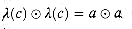 , and so on. The label we get by summarizing this infinite number of traversals of cycle c is the closure of a, defined by
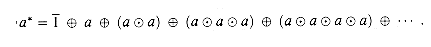
 . R0 {},
Examples of closed semirings
0 {}, min, +, ,0), which we used for shortest paths with nonnegative edge weights. (As previously noted, the min operator actually returns the greatest lower bound of its arguments.) We have also shown that a* = 0 for all a R0 {}. {-, +}, we can find a closed semiring to handle negative-weight cycles. Using min for and + for  , the reader may verify that the closure of a R {-, +} is
 on any path containing the cycle. Thus, the closed semiring to use for the Floyd-Warshall algorithm with negative edge weights is S2 = (R {-, +}, min, +, +, 0). (See Exercise 26.4-3.), 0, 1), where (i, j) = 1 if (i, j) E, and (i, j)= 0 otherwise. Here we have 0* = 1* = 1.
 A dynamic-programming algorithm for directed-path labels
: V V S. The vertices are numbered 1 through n. For each pair of vertices i, j V, we want to compute equation (26.11):  . For shortest paths, for example, we wish to compute
 be the set of paths from vertex i to vertex j with all intermediate vertices in the set { 1, 2, . . . , k}. We define
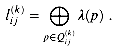
 in the Floyd-Warshall algorithm and
  in the transitive-closure algorithm. We can define
  recursively by
(26.12)
 included. This factor represents the summary of all cycles that pass through vertex k and have all other vertices in the set {1, 2, . . . , k - 1}. (When we assume no negative-weight cycles in the Floyd-Warshall algorithm,
  is 0, corresponding to
  , the weight of an empty cycle. In the transitive-closure algorithm, the empty path from k to k gives us
  . Thus, for both of these algorithms, we can ignore the factor of
  , since it is just the identity for
  .) The basis of the recursive definition is
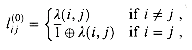 (i, j) (which is equal to
  if (i, j) is not an edge in E). If, in addition, i = j, then
  is the label of the empty path from i to i.
 in order of increasing k. It returns the matrix L(n) =
  .
.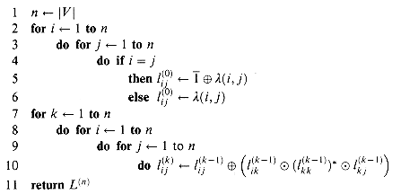
 , , and *. If we let
  , and T* represent these times, then the running time of COMPUTE-SUMMARIES is
  , which is (n3) if each of the three operations takes O(1) time.
Exercises
0 {}, min, +, , 0) and S3 = ({0, 1}, V, , 0, 1) are closed semirings. {-, +}, min, +, +, 0) is a closed semiring. What is the value of a + (- ) for a R? What about (-) + (+)? +?, 0, 1) a closed semiring?Problems
(V2) time is required to update the transitive closure after the insertion of e into G. , where ti is the time to update the transitive closure when the ith edge is inserted. Prove that your algorithm attains this time bound.-dense graphs-dense if E = (V1 + ) for some constant in the range 0 < 1. By using d-ary heaps (see Problem 7-2) in shortest-paths algorithms on -dense graphs, we can match the running times of Fibonacci-heap-based algorithms without using as complicated a data structure.(n
 ) for some constant 0 < 1? Compare these running times to the amortized costs of these operations for a Fibonacci heap.-dense directed graph G = (V, E) with no negative-weight edges in O(E) time. (Hint: Pick d as a function of .)-dense directed graph G = (V, E) with no negative-weight edges in O(V E) time.-dense directed graph G = (V, E) that may have negative-weight edges but has no negative-weight cycles. R. Let the vertex set be V = {1, 2, . . . , n}, where n = V, and assume that all edge weights w (i, j) are unique. Let T be the unique (see Exercise 24.1-6) minimum spanning tree of G. In this problem, we shall determine T by using a closed semiring, as suggested by B. M. Maggs and S. A. Plotkin. We first determine, for each pair of vertices i, j V, the minimax weight
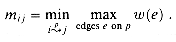 {- , }, min, max, , -) is a closed semiring.
 be the minimax weight over all paths from vertex i to vertex j with all intermediate vertices in the set {1, 2, . . . , k}.
 , where k 0. E: w(i, j) = mij}. Prove that the edges in Tm form a spanning tree of G.
Chapter notes