


Many problems of practical significance are NP-complete but are too important to abandon merely because obtaining an optimal solution is intractable. If a problem is NP-complete, we are unlikely to find a polynomial-time algorithm for solving it exactly, but this does not imply that all hope is lost. There are two approaches to getting around NP-completeness. First, if the actual inputs are small, an algorithm with exponential running time may be perfectly satisfactory. Second, it may still be possible to find near-optimal solutions in polynomial time (either in the worst case or on the average). In practice, near-optimality is often good enough. An algorithm that returns near-optimal solutions is called an approximation algorithm. This chapter presents polynomial-time approximation algorithms for several NP-complete problems.
Performance bounds for approximation algorithms
Assume that we are working on an optimization problem in which each potential solution has a positive cost, and that we wish to find a near-optimal solution. Depending on the problem, an optimal solution may be defined as one with maximum possible cost or one with minimum possible cost; the problem may be a maximization or a minimization problem.
We say that an approximation algorithm for the problem has a ratio bound of
This definition applies for both minimization and maximization problems. For a maximization problem, 0 < C
Sometimes, it is more convenient to work with a measure of relative error. For any input, the relative error of the approximation algorithm is defined to be
where, as before, C* is the cost of an optimal solution and C is the cost of the solution produced by the approximation algorithm. The relative error is always nonnegative. An approximation algorithm has a relative error bound of
It follows from the definitions that the relative error bound can be bounded as a function of the ratio bound:
(For a minimization problem, this is an equality, whereas for a maximization problem, we have
For many problems, approximation algorithms have been developed that have a fixed ratio bound, independent of n. For such problems, we simply use the notation
For other problems, computer scientists have been unable to devise any polynomial-time approximation algorithm having a fixed ratio bound. For such problems, the best that can be done is to let the ratio bound grow as a function of the input size n. An example of such a problem is the set-cover problem presented in Section 37.3.
Some NP-complete problems allow approximation algorithms that can achieve increasingly smaller ratio bounds (or, equivalently, increasingly smaller relative error bounds) by using more and more computation time. That is, there is a trade-off between computation time and the quality of the approximation. An example is the subset-sum problem studied in Section 37.4. This situation is important enough to deserve a name of its own.
An approximation scheme for an optimization problem is an approximation algorithm that takes as input not only an instance of the problem, but also a value
The running time of a polynomial-time approximation scheme should not increase too rapidly as
We say that an approximation scheme is a fully polynomial-time approximation scheme if its running time is polynomial both in 1/
Chapter outline
The first three sections of this chapter present some examples of polynomial-time approximation algorithms for NP-complete problems, and the last section presents a fully polynomial-time approximation scheme. Section 37.1 begins with a study of the vertex-cover problem, an NP-complete minimization problem that has an approximation algorithm with a ratio bound of 2. Section 37.2 presents an approximation algorithm with ratio bound 2 for the case of the traveling-salesman problem in which the cost function satisfies the triangle inequality. It also shows that without triangle inequality, an
The vertex-cover problem was defined and proved NP-complete in Section 36.5.2. A vertex cover of an undirected graph G = (V,E) is a subset V'
The vertex-cover problem is to find a vertex cover of minimum size in a given undirected graph. We call such a vertex cover an optimal vertex cover. This problem is NP-hard, since the related decision problem is NP-complete, by Theorem 36.12.
Even though it may be difficult to find an optimal vertex cover in a graph G, however, it is not too hard to find a vertex cover that is near-optimal. The following approximation algorithm takes as input an undirected graph G and returns a vertex cover whose size is guaranteed to be no more than twice the size of an optimal vertex cover.
Figure 37.1 illustrates the operation of APPROX-VERTEX-COVER. The variable C contains the vertex cover being constructed. Line 1 initializes C to the empty set. Line 2 sets E' to be a copy of the edge set E[G] of the graph. The loop on lines 3-6 repeatedly picks an edge (u, v) from E', adds its endpoints u and v to C, and deletes all edges in E' that are covered by either u or v. The running time of this algorithm is O(E), using an appropriate data structure for representing E'.
Theorem 37.1
APPROX-VERTEX-COVER has a ratio bound of 2.
Proof The set C of vertices that is returned by APPROX-VERTEX-COVER is a vertex cover, since the algorithm loops until every edge in E[G] has been covered by some vertex in C.
To see that APPROX-VERTEX-COVER returns a vertex cover that is at most twice the size of an optimal cover, let A denote the set of edges that were picked in line 4 of APPROX-VERTEX-COVER. No two edges in A share an endpoint, since once an edge is picked in line 4, all other edges that are incident on its endpoints are deleted from E' in line 6. Therefore, each execution of line 5 adds two new vertices to C, and |C| = 2 |A|. In order to cover the edges in A, however, any vertex cover--in particular, an optimal cover C*--must include at least one endpoint of each edge in A. Since no two edges in A share an endpoint, no vertex in the cover is incident on more than one edge in A. Therefore, |A|
37.1-1
Given an example of a graph for which APPROX-VERTEX-COVER always yields a suboptimal solution.
37.1-2
Professor Nixon proposes the following heuristic to solve the vertex-cover problem. Repeatedly select a vertex of highest degree, and remove all of its incident edges. Give an example to show that the professor's heuristic does not have a ratio bound of 2.
37.1-3
Give an efficient greedy algorithm that finds an optimal vertex cover for a tree in linear time.
37.1-4
From the proof of Theorem 36.12, we know that the vertex-cover problem and the NP-complete clique problem are complementary in the sense that an optimal vertex cover is the complement of a maximum-size clique in the complement graph. Does this relationship imply that there is an approximation algorithm with constant ratio bound for the clique problem? Justify your answer.
In the traveling-salesman problem introduced in Section 36.5.5, we are given a complete undirected graph G = (V, E) that has a nonnegative integer cost c(u, v) associated with each edge (u, v)
In many practical situations, it is always cheapest to go directly from a place u to a place w; going by way of any intermediate stop v can't be less expensive. Putting it another way, cutting out an intermediate stop never increases the cost. We formalize this notion by saying that the cost function c satisfies the triangle inequality if for all vertices u, v, w
The triangle inequality is a natural one, and in many applications it is automatically satisfied. For example, if the vertices of the graph are points in the plane and the cost of traveling between two vertices is the ordinary euclidean distance between them, then the triangle inequality is satisfied.
As Exercise 37.2-1 shows, restricting the cost function to satisfy the triangle inequality does not alter the NP-completeness of the traveling- salesman problem. Thus, it is unlikely that we can find a polynomial-time algorithm for solving this problem exactly. We therefore look instead for good approximation algorithms.
In Section 37.2.1, we examine an approximation algorithm for the traveling-salesman problem with triangle inequality that has a ratio bound of 2. In Section 37.2.2, we show that without triangle inequality, an approximation algorithm with constant ratio bound does not exist unless P = NP.
The following algorithm computes a near-optimal tour of an undirected graph G, using the minimum-spanning-tree algorithm MST-PRIM from Section 24.2. We shall see that when the cost function satisfies the triangle inequality, the tour that this algorithm returns is no worse than twice as long as an optimal tour.
Recall from Section 13.1 that a preorder tree walk recursively visits every vertex in the tree, listing a vertex when it is first encountered, before any of its children are visited.
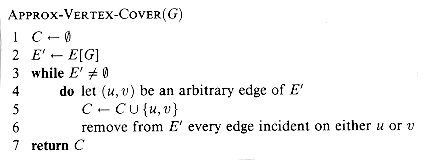
Figure 37.2 illustrates the operation of APPROX-TSP-TOUR. Part (a) of the figure shows the given set of vertices, and part (b) shows the minimum spanning tree T grown from root vertex a by MST-PRIM. Part (c) shows how the vertices are visited by a preorder walk of T, and part (d) displays the corresponding tour, which is the tour returned by APPROX-TSP-TOUR. Part (e) displays an optimal tour, which is about 23% shorter.
The running time of APPROX-TSP-TOUR is
Theorem 37.2
APPROX-TSP-TOUR is an approximation algorithm with a ratio bound of 2 for the traveling-salesman problem with triangle inequality.
Proof Let H* denote an optimal tour for the given set of vertices. An equivalent statement of the theorem is that c(H)
A full walk of T lists the vertices when they are first visited and also whenever they are returned to after a visit to a subtree. Let us call this walk W. The full walk of our example gives the order
Since the full walk traverses every edge of T exactly twice, we have
Equations (37.4) and (37.5) imply that
and so the cost of W is within a factor of 2 of the cost of an optimal tour.
Unfortunately, W is generally not a tour, since it visits some vertices more than once. By the triangle inequality, however, we can delete a visit to any vertex from W and the cost does not increase. (If a vertex v is deleted from W between visits to u and w, the resulting ordering specifies going directly from u to w.) By repeatedly applying this operation, we can remove from W all but the first visit to each vertex. In our example, this leaves the ordering
This ordering is the same as that obtained by a preorder walk of the tree T. Let H be the cycle corresponding to this preorder walk. It is a hamiltonian cycle, since every vertex is visited exactly once, and in fact it is the cycle computed by APPROX-TSP-TOUR. Since H is obtained by deleting vertices from the full walk W, we have
Combining inequalities (37.6) and (37.7) completes the proof.
In spite of the nice ratio bound provided by Theorem 37.2, APPROX-TSP-TOUR is usually not the best practical choice for this problem. There are other approximation algorithms that typically perform much better in practice (see the references at the end of this chapter).
If we drop the assumption that the cost function c satisfies the triangle inequality, good approximate tours cannot be found in polynomial time unless P = NP.
Theorem 37.3
If P
Proof The proof is by contradiction. Suppose to the contrary that for some number
Let G = (V, E) be an instance of the hamiltonian-cycle problem. We wish to determine efficiently whether G contains a hamiltonian cycle by making use of the hypothesized approximation algorithm A. We turn G into an instance of the traveling-salesman problem as follows. Let G' = (V, E') be the complete graph on V; that is,
Assign an integer cost to each edge in E' as follows:
Representations of G' and c can be created from a representation of G in time polynomial in |V| and |E|.
Now, consider the traveling-salesman problem (G', c). If the originalgraph G has a hamiltonian cycle H, then the cost function c assigns to each edge of H a cost of 1, and so (G', c) contains a tour of cost |V| On the other hand, if G does not contain a hamiltonian cycle, then any tour of G' must use some edge not in E. But any tour that uses an edge not in E has a cost of at least
Because edges not in G are so costly, there is a large gap between the cost of a tour that is a hamiltonian cycle in G (cost |V|) and the cost of any other tour (cost greater than
What happens if we apply the approximation algorithm A to the traveling-salesman problem (G', c)? Because A is guaranteed to return a tour of cost no more than
37.2-1
Show how in polynomial time we can transform one instance of the traveling-salesman problem into another instance whose cost function satisfies the triangle inequality. The two instances must have the same set of optimal tours. Explain why such a polynomial-time transformation does not contradict Theorem 37.3, assuming that P
37.2-2
Consider the following closest-point heuristic for building an approximate traveling-salesman tour. Begin with a trivial cycle consisting of a single arbitrarily chosen vertex. At each step, identify the vertex u that is not on the cycle but whose distance to any vertex on the cycle is minimum. Suppose that the vertex on the cycle that is nearest u is vertex v. Extend the cycle to include u by inserting u just after v. Repeat until all vertices are on the cycle. Prove that this heuristic returns a tour whose total cost is not more than twice the cost of an optimal tour.
37.2-3
The bottleneck traveling-salesman problem is the problem of finding the hamiltonian cycle such that the length of the longest edge in the cycle is minimized. Assuming that the cost function satisfies the triangle inequality, show that there exists a polynomial-time approximation algorithm with ratio bound 3 for this problem. (Hint: Show recursively that we can visit all the nodes in a minimum spanning tree exactly once by taking a full walk of the tree and skipping nodes, but without skipping more than 2 consecutive intermediate nodes.)
37.2-4
Suppose that the vertices for an instance of the traveling-salesman problem are points in the plane and that the cost c(u, v) is the euclidean distance between points u and v. Show that an optimal tour never crosses itself.
The set-covering problem is an optimization problem that models many resource-selection problems. It generalizes the NP-complete vertex-cover problem and is therefore also NP-hard. The approximation algorithm developed to handle the vertex-cover problem doesn't apply here, however, and so we need to try other approaches. We shall examine a simple greedy heuristic with a logarithmic ratio bound. That is, as the size of the instance gets larger, the size of the approximate solution may grow, relative to the size of an optimal solution. Because the logarithm function grows rather slowly, however, this approximation algorithm may nonetheless give useful results.
An instance
We say that a subset
We say that any
The set-covering problem is an abstraction of many commonly arising combinatorial problems. As a simple example, suppose that X represents a set of skills that are needed to solve a problem and that we have a given set of people available to work on the problem. We wish to form a committee, containing as few people as possible, such that for every requisite skill in X, there is a member of the committee having that skill. In the decision version of the set-covering problem, we ask whether or not a covering exists with size at most k, where k is an additional parameter specified in the problem instance. The decision version of the problem is NP-complete, as Exercise 37.3-2 asks you to show.
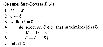
The greedy method works by picking, at each stage, the set S that covers the most remaining uncovered elements.
In the example of Figure 37.3, GREEDY-SET-COVER adds to
The algorithm works as follows. The set U contains, at each stage, the set of remaining uncovered elements. The set
The algorithm GREEDY-SET-COVER can easily be implemented to run in time polynomial in
We now show that the greedy algorithm returns a set cover that is not too much larger than an optimal set cover. For convenience, in this chapter we denote the dth harmonic number
Theorem 37.4
GREEDY-SET-COVER has a ratio bound
Proof The proof proceeds by assigning a cost to each set selected by the algorithm, distributing this cost over the elements covered for the first time, and then using these costs to derive the desired relationship between the size of an optimal set cover
The algorithm finds a solution
The remainder of the proof rests on the following key inequality, which we shall prove shortly. For any set S belonging to the family
From inequalities (37.9) and (37.10), it follows that
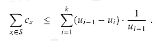
proving the theorem. It thus remains only to prove inequality (37.10). For any set
be the number of elements in S remaining uncovered after S1, S2, . . . , Si have been selected by the algorithm. We define u0 = |S| to be the number of elements of S, which are all initially uncovered. Let k be the least index such that uk = 0, so that every element in S is covered by at least one of the sets S1, S2, . . . , Sk. Then, ui-1
Observe that
because the greedy choice of Si guarantees that S cannot cover more new elements than Si does (otherwise, S would have been chosen instead of Si). Consequently, we obtain
For integers a and b, where a < b, we have
Using this inequality, we obtain the telescoping sum
since H(0) = 0. This completes the proof of inequality (37.10).
Corollary 37.5
GREEDY-SET-COVER has a ratio bound of (ln |X| + 1).
Proof Use inequality (3.12) and Theorem 37.4.
In some applications, max
37.3-1
Consider each of the following words as a set of letters: {arid, dash, drain, heard, lost, nose, shun, slate, snare, thread}. Show which set cover GREEDY-SET-COVER produces when ties are broken in favor of the word that appears first in the dictionary.
37.3-2
Show that the decision version of the set-covering problem is NP-complete by reduction from the vertex-cover problem.
37.3-3
Show how to implement GREEDY-SET-COVER in such a way that it runs in time
37.3-4
Show that the following weaker form of Theorem 37.4 is trivially true:
37.3-5
Create a family of set-cover instances demonstrating that GREEDY-SET-COVER can return a number of different solutions that is exponential in the size of the instance. (Different solutions result from ties being broken differently in the choice of S in line 4.)
An instance of the subset-sum problem is a pair (S, t), where S is a set {x1, x2, . . . , xn} of positive integers and t is a positive integer. This decision problem asks whether there exists a subset of S that adds up exactly to the target value t. This problem is NP-complete (see Section 36.5.3).
The optimization problem associated with this decision problem arises in practical applications. In the optimization problem, we wish to find a subset of {x1, x2, . . . , xn} whose sum is as large as possible but not larger than t. For example, we may have a truck that can carry no more than t pounds, and n different boxes to ship, the ith of which weighs xi pounds. We wish to fill the truck as full as possible without exceeding the given weight limit.
In this section, we present an exponential-time algorithm for this optimization problem and then show how to modify the algorithm so that it becomes a fully polynomial-time approximation scheme. (Recall that a fully polynomial-time approximation scheme has a running time that is polynomial in 1/
If L is a list of positive integers and x is another positive integer, then we let L + x denote the list of integers derived from L by increasing each element of L by x. For example, if L =
We use an auxiliary procedure MERGE-LISTS(L, L') that returns the sorted list that is the merge of its two sorted input lists L and L'. Like the MERGE procedure we used in merge sort (Section 1.3.1), MERGE-LISTS runs in time O(|L| + |L'|). (We omit giving pseudocode for MERGE-LISTS.) The procedure EXACT-SUBSET-SUM takes an input set S = {x1, x2, . . . , xn} and a target value t.
Let Pi denote the set of all values that can be obtained by selecting a (possibly empty) subset of {x1, x2, . . . , xi} and summing its members. For example, if S = {1, 4, 5}, then
Given the identity
we can prove by induction on i (see Exercise 37.4-1) that the list Li is a sorted list containing every element of Pi whose value is not more than t. Since the length of Li can be as much as 2i, EXACT-SUBSET-SUM is an exponential-time algorithm in general, although it is a polynomial-time algorithm in the special cases in which t is polynomial in |S| or all of the numbers in S are bounded by a polynomial in |S|.
We can derive a fully polynomial-time approximation scheme for the subset-sum problem by "trimming" each list Li after it is created. We use a trimming parameter
or, equivalently,
We can think of such a z as "representing" y in the new list L'. Each y is represented by a z such that the relative error of z, with respect to y, is at most
then we can trim L to obtain
where the deleted value 11 is represented by 10, the deleted values 21 and 22 are represented by 20, and the deleted value 24 is represented by 23. It is important to remember that every element of the trimmed version of the list is also an element of the original version of the list. Trimming a list can dramatically decrease the number of elements in the list while keeping a close (and slightly smaller) representative value in the list for each element deleted from the list.
The following procedure trims an input list L =
The elements of L are scanned in increasing order, and a number is put into the returned list L' only if it is the first element of L or if it cannot be represented by the most recent number placed into L'.
Given the procedure TRIM, we can construct our approximation scheme as follows. This procedure takes as input a set S = {x1, x2, . . . , xn} of n integers (in arbitrary order), a target integer t, and an "approximation parameter"
Line 2 initializes the list L0 to be the list containing just the element 0. The loop in lines 3-6 has the effect of computing Li as a sorted list containing a suitably trimmed version of the set Pi, with all elements larger than t removed. Since Li is created from Li-1, we must ensure that the repeated trimming doesn't introduce too much inaccuracy. In a moment, we shall see that APPROX-SUBSET-SUM returns a correct approximation if one exists.
As an example, suppose we have the instance
with t = 308 and
The algorithm returns z = 302 as its answer, which is well within
Theorem 37.6
APPROX-SUBSET-SUM is a fully polynomial-time approximation scheme for the subset-sum problem.
Proof The operations of trimming Li in line 5 and removing from Li every element that is greater than t maintain the property that every element of Li is also a member of Pi. Therefore, the value z returned in line 8 is indeed the sum of some subset of S. It remains to show that it is not smaller than 1 -
To show that the relative error of the returned answer is small, note that when list Li is trimmed, we introduce a relative error of at most
If y*
the largest such z is the value returned by APPROX-SUBSET-SUM. Since it can be shown that
the function (1 -
and thus,
Therefore, the value z returned by APPROX-SUBSET-SUM is not smaller than 1 -
To show that this is a fully polynomial-time approximation scheme, we derive a bound on the length of Li. After trimming, successive elements z and z' of Li must have the relationship z/z' > 1/(1 -
using equation (2.10). This bound is polynomial in the number n of input values given, in the number of bits 1g t needed to represent t, and in 1/
37.4-1
Prove equation (37.11).
37.4-2
Prove equations (37.12) and (37.13).
37.4-3
How would you modify the approximation scheme presented in this section to find a good approximation to the smallest value not less than t that is a sum of some subset of the given input list?
37-1 Bin packing
Suppose that we are given a set of n objects, where the the size si of the ith object satisfies 0 < si < 1. We wish to pack all the objects into the minimum number of unit-size bins. Each bin can hold any subset of the objects whose total size does not exceed 1.
a. Prove that the problem of determining the minimum number of bins required is NP-hard. (Hint: Reduce from the subset-sum problem.)
The first-fit heuristic takes each object in turn and places it into the first bin that can accommodate it. Let
b. Argue that the optimal number of bins required is at least
c. Argue that the first-fit heuristic leaves at most one bin less than half full.
d. Prove that the number of bins used by the first-fit heuristic is never more than
e. Prove a ratio bound of 2 for the first-fit heuristic.
f. Give an efficient implementation of the first-fit heuristic, and analyze its running time.
37-2 Approximating the size of a maximum clique
Let G = (V, E) be an undirected graph. For any k
a. Prove that the size of the maximum clique in G(k) is equal to the kth power of the size of the maximum clique in G.
b. Argue that if there is an approximation algorithm that has a constant ratio bound for finding a maximum-size clique, then there is a fully polynomial-time approximation scheme for the problem.
37-3 Weighted set-covering problem
Suppose that we generalize the set-covering problem so that each set Si in the family
Show that the greedy set-covering heuristic can be generalized in a natural manner to provide an approximate solution for any instance of the weighted set-covering problem. Show that your heuristic has a ratio bound of H(d), where d is the maximum size of any set Si.
There is a wealth of literature on approximation algorithms. A good place to start is Garey and Johnson [79]. Papadimitriou and Steiglitz [154] also have an excellent presentation of approximation algorithms. Lawler, Lenstra, Rinnooy Kan, and Shmoys [133] provide an extensive treatment of the traveling-salesman problem.
Papadimitriou and Steiglitz attribute the algorithm APPROX-VERTEX-COVER to F. Gavril and M. Yannakakis. The algorithm APPROX-TSP-TOUR appears in an excellent paper by Rosenkrantz, Stearns, and Lewis [170]. Theorem 37.3 is due to Sahni and Gonzalez [172]. The analysis of the greedy heuristic for the set-covering problem is modeled after the proof published by Chvátal [42] of a more general result; this basic result as presented here is due to Johnson [113] and Lovász [141]. The algorithm APPROX-SUBSET-SUM and its analysis are loosely modeled after related approximation algorithms for the knapsack and subset-sum problem by Ibarra and Kim [111].
 (n) if for any input of size n, the cost C of the solution produced by the approximation algorithm is within a factor of (n) of the cost C* of an optimal solution:
(37.1)
 C*, and the ratio C*/C gives the factor by which the cost of an optimal solution is larger than the cost of the approximate solution. Similarly, for a minimization problem, 0 < C* C, and the ratio C/C* gives the factor by which the cost of the approximate solution is larger than the cost of an optimal solution. Since all solutions are assumed to have positive cost, these ratios are always well defined. The ratio bound of an approximation algorithm is never less than 1, since C/C* < 1 implies C*/C > 1. An optimal algorithm has ratio bound 1, and an approximation algorithm with a large ratio bound may return a solution that is very much worse than optimal.
 (n) if
(37.2)
(n) (n) - 1.(37.3)
(n) = ((n) - 1) / (n), which satisfies inequality (37.3) since (n)  1.) or , indicating no dependence on n. > 0 such that for any fixed , the scheme is an approximation algorithm with relative error bound . We say that an approximation scheme is a polynomial-time approximation scheme if for any fixed > 0, the scheme runs in time polynomial in the size n of its input instance. decreases. Ideally, if decreases by a constant factor, the running time to achieve the desired approximation should not increase by more than a constant factor. In other words, we would like the running time to be polynomial in 1/ as well as in n. and in the size n of the input instance, where is the relative error bound for the scheme. For example, the scheme might have a running time of (1/)2n3. With such a scheme, any constant-factor decrease in can be achieved with a corresponding constant-factor increase in the running time.-approximation algorithm cannot exist unless P = NP. In Section 37.3, we show how a greedy method can be used as an effective approximation algorithm for the set-covering problem, obtaining a covering whose cost is at worst a logarithmic factor larger than the optimal cost. Finally, Section 37.4 presents a fully polynomial-time approximation scheme for the subset-sum problem.
37.1 The vertex-cover problem
 V such that if (u,v) is an edge of G, then either u V' or v V' (or both). The size of a vertex cover is the number of vertices in it.
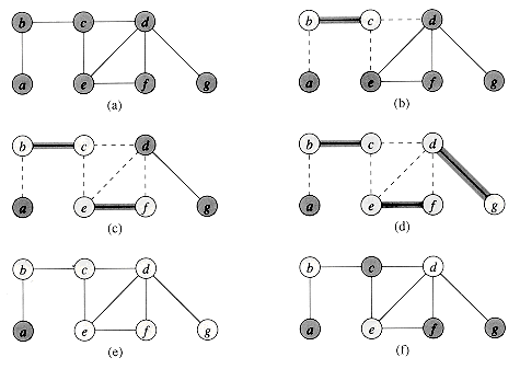
Figure 37.1 The operation of APPROX-VERTEX-COVER. (a) The input graph G, which has 7 vertices and 8 edges. (b) The edge (b,c), shown heavy, is the first edge chosen by APPROX-VERTEX-COVER. Vertices b and c, shown lightly shaded, are added to the set A containing the vertex cover being created. Edges (a, b), (c, e), and (c,d), shown dashed, are removed since they are now covered by some vertex in A. (c) Edge (e, f) is added to A. (d) Edge (d,g) is added to A. (e) The set A, which is the vertex cover produced by APPROX-VERTEX-COVER, contains the six vertices b, c, d, e, f, g. (f) The optimal vertex cover for this problem contains only three vertices: b, d, and e.
 |C*|, and |C| 2 |C*|, proving the theorem.
 Exercises
37.2 The traveling-salesman problem
E, and we must find a hamiltonian cycle (a tour) of G with minimum cost. As an extension of our notation, let c(A) denote the total cost of the edges in the subset A E: V,
V,c(u, w)
c(u, v) + c(v, w).37.2.1 The traveling-salesman problem with triangle inequality
APPROX-TSP-TOUR(G, c)
1 select a vertex r
V[G] to be a "root" vertex2 grow a minimum spanning tree T for G from root r
using MST-PRIM(G, c, r)
3 let L be the list of vertices visited in a preorder tree walk of T
4 return the hamiltonian cycle H that visits the vertices in the order L
 (E) = (V2), since the input is a complete graph (see Exercise 24.2-2). We shall now show that if the cost function for an instance of the traveling-salesman problem satisfies the triangle inequality, then APPROX-TSP-TOUR returns a tour whose cost is not more than twice the cost of an optimal tour. 2c(H*), where H is the tour returned by APPROX-TSP-TOUR. Since we obtain a spanning tree by deleting any edge from a tour, if T is a minimum spanning tree for the given set of vertices, then
c(T)
c(H*) .(37.4)
a, b, c, b, h, b, a, d, e, f, e, g, e, d, a.
c(W) = 2c(T) .
(37.5)
c(W)
2c(H*),(37.6)

Figure 37.2 The operation of APPROX-TSP-TOUR. (a) The given set of points, which lie on vertices of an integer grid. For example, f is one unit to the right and two units up from h. The ordinary euclidean distance is used as the cost function between two points. (b) A minimum spanning tree T of these points, as computed by MST-PRIM. Vertex a is the root vertex. The vertices happen to be labeled in such a way that they are added to the main tree by MST-PRIM in alphabetical order. (c) A walk of T, starting at a. A full walk of the tree visits the vertices in the order a, b, c, b, h, b, a, d, e, f, e, g, e, d, a. A preorder walk of T lists a vertex just when it is first encountered, yielding the ordering a, b, c, h, d, e, f, g. (d) A tour of the vertices obtained by visiting the vertices in the order given by the preorder walk. This is the tour H returned by APPROX-TSP-TOUR. Its total cost is approximately 19.074. (e) An optimal tour H* for the given set of vertices. Its total cost is approximately 14.715.
a, b, c, h, d, e, f, g .
c(H)
c(W).(37.7)
37.2.2 The general traveling-salesman problem
 NP and 1, there is no polynomial-time approximation algorithm with ratio bound for the general traveling-salesman problem. 1, there is a polynomial-time approximation algorithm A with ratio bound . Without loss of generality, we assume that is an integer, by rounding it up if necessary. We shall then show how to use A to solve instances of the hamiltonian-cycle problem (defined in Section 36.5.5) in polynomial time. Since the hamiltonian-cycle problem is NP-complete, by Theorem 36.14, solving it in polynomial time implies that P = NP, by Theorem 36.4.
E' = {(u, v): u, v V and u v}.
(
|V| + 1) + (|V| - 1) > |V| .|V|). times the cost of an optimal tour, if G contains a hamiltonian cycle, then A must return it. If G has no hamiltonian cycle, then A returns a tour of cost more than |V|. Therefore, we can use A to solve the hamiltonian-cycle problem in polynomial time. Exercises
NP.37.3 The set-covering problem
 of the set-covering problem consists of a finite set X and a family
  of subsets of X, such that every element of X belongs to at least one subset in
  :
:
 covers its elements. The problem is to find a minimum-size subset
  whose members cover all of X:
(37.8)
 satisfying equation (37.8) covers X. Figure 37.3 illustrates the problem.
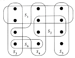
Figure 37.3 An instance
 of the set-covering problem, where X consists of the 12 black points and
  . A minimum-size set cover is
  . The greedy algorithm produces a cover of size 4 by selecting the sets S1,S4,S5, and S3 in order.
A greedy approximation algorithm
 the sets Sl, S4, S5, S3 in order.
 contains the cover being constructed. Line 4 is the greedy decision-making step. A subset S is chosen that covers as many uncovered elements as possible (with ties broken arbitrarily). After S is selected, its elements are removed from U, and S is placed in
  . When the algorithm terminates, the set
  contains a subfamily of
  that covers X.
 . Since the number of iterations of the loop on lines 3-6 is at most min
  , and the loop body can be implemented to run in time
  , there is an implementation that runs in time
 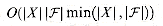 . Exercise 37.3-3 asks for a linear- time algorithm.
Analysis
 (see Section 3.1) by H(d) .
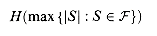
 and the size of the set cover
  returned by the algorithm. Let Si denote the ith subset selected by GREEDY-SET-COVER; the algorithm incurs a cost of 1 when it adds Si to
  . We spread this cost of selecting Si evenly among the elements covered for the first time by Si. Let cx denote the cost allocated to element x, for each x X. Each element is assigned a cost only once, when it is covered for the first time. If x is covered for the first time by Si, then
 of total cost
  , and this cost has been spread out over the elements of X. Therefore, since the optimal cover
  also covers X, we have
(37.9)
 ,
,
(37.10)

 , let
, let ui, and ui-1 - ui elements of S are covered for the first time by Si, for i = 1, 2, . . . , k. Thus,
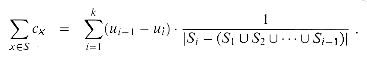


 is a small constant, and so the solution returned by GREEDY-SET-COVER is at most a small constant times larger than optimal. One such application occurs when this heuristic is used to obtain an approximate vertex cover for a graph whose vertices have degree at most 3. In this case, the solution found by GREEDY-SET-COVER is not more than H(3) = 11/6 times as large as an optimal solution, a performance guarantee that is slightly better than that of APPROX-VERTEX-COVER.
Exercises
 .
.
37.4 The subset-sum problem
as well as in n.)An exponential-time algorithm
 1, 2, 3, 5, 9
 , then L + 2 = 3, 4, 5, 7, 11. We also use this notation for sets, so that
S + x = {s + x : s S} .EXACT-SUBSET-SUM(S, t)
1 n
 |S|
|S|2 L0
03 for i
1 to n4 do Li
MERGE-LISTS(Li-1, Li-1 + xi)5 remove from Li every element that is greater than t
6 return the largest element in Ln
P1 = {0, 1} ,P2 = {0, 1, 4, 5} ,P3 = {0, 1, 4, 5, 6, 9, 10} .
(37.11)
A fully polynomial-time approximation scheme
 such that 0 < < 1. To trim a list L by means to remove as many elements from L as possible, in such a way that if L'is the result of trimming L, then for every element y that was removed from L, there is an element z y still in L' such that
(1 -
)y z y .. For example, if = 0.1 andL =
10, 11, 12, 15, 20, 21, 22, 23, 24, 29,L' =
10, 12, 15, 20, 23, 29,y1, y2, . . . , ym in time (m), assuming that L is sorted into nondecreasing order. The output of the procedure is a trimmed, sorted list.TRIM(L,
)1 m
|L|2 L'
<y1>3 last
<y1>4 for i
2 to m5 do if last < (1 -
)yi6 then append yi onto the end of L'
7 last
yi8 return L'
, where 0 < < 1.APPROX-SUBSET-SUM(S, t,
)1 n
|S|2 L0
03 for i
1 to n4 do Li
MERGE-LISTS(Li-1, Li-1 + xi)5 Li
TRIM(Li, / n)6 remove from Li every element that is greater than t
7 let z be the largest value in Ln
8 return z
L =
104, 102, 201, 101 = 0.20. The trimming parameter is / 4 = 0.05. APPROX-SUBSET-SUM computes the following values on the indicated lines:line 2: L0 =
0 ,line 4: L1 =
0, 104 ,line 5: L1 =
0, 104 ,line 6: L1 =
0, 104 ,line 4: L2 =
0, 102, 104, 206 ,line 5: L2 =
0, 102, 206 ,line 6: L2 =
0, 102, 206 ,line 4: L3 =
0,102, 201, 206, 303, 407 ,line 5: L3 =
0,102, 201, 303, 407 ,line 6: L3 =
0, 102, 201, 303 ,line 4: L4 =
0, 101, 102, 201, 203, 302, 303, 404 ,line 5: L4 =
0,101, 201, 302, 404 ,line 6: L4 =
0,101, 201, 302 . = 20% of the optimal answer 307 = 104 + 102 + 101; in fact, it is within 2%. times an optimal solution. (Note that because the subset-sum problem is a maximization problem, equation (37.2) is equivalent to C*(1-) C.) We must also show that the algorithm runs in polynomial time./n between the representative values remaining and the values before trimming. By induction on i, it can be shown that for every element y in Pi that is at most t, there is a z Li such that(1 -
/n)iy z y.(37.12)
Pn denotes an optimal solution to the subset-sum problem, then there is a z Ln such that(1 -
/n)ny* z y*;(37.13)
 /n)n increases with n, so that n > 1 implies
1 -
<(1 - /n)n,(1 -
)y* z. times the optimal solution y*./n). That is, they must differ by a factor of at least 1/(1 - /n). Therefore, the number of elements in each Li is at most . Since the running time of APPROX-SUBSET-SUM is polynomial in the length of the Li, APPROX-SUBSET-SUM is a fully polynomial-time approximation scheme.
 Exercises
Problems
 .
. S
S .2S. 1, define G(k) to be the undirected graph (V(k), E(k), where V(k) is the set of all ordered k-tuples of vertices from V and E(k) is defined so that (v1,v2, . . . , vk) is adjacent to (w1, w2, . . . , wk) if and only if for some i, vertex vi is adjacent to wi in G.
 has an associated weight wi and the weight of a cover
  is
is  Sicwi. We wish to determine a minimum-weight cover. (Section 37.3 handles the case in which wi = 1 for all i.)
Chapter notes