


In the previous chapters, we studied the representation of simple data structures using an array and a sequential mapping. These representations had the property that successive nodes of the data object were stored a fixed distance apart. Thus, (i) if the element aij of a table was stored at location Lij, then ai,j+1 was at the location Lij + c for some constant c; (ii) if the ith node in a queue was at location Li, then the i + 1- st node was at location Li + c mod n for the circular representation; (iii) if the topmost node of a stack was at location LT, then the node beneath it was at location LT - c, etc. These sequential storage schemes proved adequate given the functions one wished to perform (access to an arbitrary node in a table, insertion or deletion of nodes within a stack or queue).
However when a sequential mapping is used for ordered lists, operations such as insertion and deletion of arbitrary elements become expensive. For example, consider the following list of all of the three letter English words ending in AT:
(BAT, CAT, EAT, FAT, HAT, JAT, LAT, MAT, OAT, PAT, RAT, SAT, TAT, VAT, WAT)
To make this list complete we naturally want to add the word GAT, which means gun or revolver. If we are using an array to keep this list, then the insertion of GAT will require us to move elements already in the list either one location higher or lower. We must either move HAT, JAT, LAT, ..., WAT or else move BAT, CAT, EAT and FAT. If we have to do many such insertions into the middle, then neither alternative is attractive because of the amount of data movement. On the other hand, suppose we decide to remove the word LAT which refers to the Latvian monetary unit. Then again, we have to move many elements so as to maintain the sequential representation of the list.
When our problem called for several ordered lists of varying sizes, sequential representation again proved to be inadequate. By storing each list in a different array of maximum size, storage may be wasted. By maintaining the lists in a single array a potentially large amount of data movement is needed. This was explicitly observed when we represented several stacks, queues, polynomials and matrices. All these data objects are examples of ordered lists. Polynomials are ordered by exponent while matrices are ordered by rows and columns. In this chapter we shall present an alternative representation for ordered lists which will reduce the time needed for arbitrary insertion and deletion.
An elegant solution to this problem of data movement in sequential representations is achieved by using linked representations. Unlike a sequential representation where successive items of a list are located a fixed distance apart, in a linked representation these items may be placed anywhere in memory. Another way of saying this is that in a sequential representation the order of elements is the same as in the ordered list, while in a linked representation these two sequences need not be the same. To access elements in the list in the correct order, with each element we store the address or location of the next element in that list. Thus, associated with each data item in a linked representation is a pointer to the next item. This pointer is often referred to as a link. In general, a node is a collection of data, DATA1, ...,DATAn and links LINK1, ...,LINKm. Each item in a node is called a field. A field contains either a data item or a link.
Figure 4.1 shows how some of the nodes of the list we considered before may be represented in memory by using pointers. The elements of the list are stored in a one dimensional array called DATA. But the elements no longer occur in sequential order, BAT before CAT before EAT, etc. Instead we relax this restriction and allow them to appear anywhere in the array and in any order. In order to remind us of the real order, a second array, LINK, is added. The values in this array are pointers to elements in the DATA array. Since the list starts at DATA(8) = BAT, let us set a variable F = 8. LINK(8) has the value 3, which means it points to DATA(3) which contains CAT. The third element of the list is pointed at by LINK(3) which is EAT. By continuing in this way we can list all the words in the proper order.
We recognize that we have come to the end when LINK has a value of zero.
Some of the values of DATA and LINK are undefined such as DATA(2), LINK(2), DATA(5), LINK(5), etc. We shall ignore this for the moment.
It is customary to draw linked lists as an ordered sequence of nodes with links being represented by arrows as in figure 4.2. Notice that we do not explicitly put in the values of the pointers but simply draw arrows to indicate they are there. This is so that we reinforce in our own mind the facts that (i) the nodes do not actually reside in sequential locations, and that (ii) the locations of nodes may change on different runs. Therefore, when we write a program which works with lists, we almost never look for a specific address except when we test for zero.
Let us now see why it is easier to make arbitrary insertions and deletions using a linked list rather than a sequential list. To insert the data item GAT between FAT and HAT the following steps are adequate:
(i) get a node which is currently unused; let its address be X;
(ii) set the DATA field of this node to GAT;
(iii) set the LINK field of X to point to the node after FAT which contains HAT;
(iv) set the LINK field of the node containing FAT to X.
Figure 4.3a shows how the arrays DATA and LINK will be changed after we insert GAT. Figure 4.3b shows how we can draw the insertion using our arrow notation. The new arrows are dashed. The important thing to notice is that when we insert GAT we do not have to move any other elements which are already in the list. We have overcome the need to move data at the expense of the storage needed for the second field, LINK. But we will see that this is not too severe a penalty.
Now suppose we want to delete GAT from the list. All we need to do is find the element which immediately precedes GAT, which is FAT, and set LINK(9) to the position of HAT which is 1. Again, there is no need to move the data around. Even though the LINK field of GAT still contains a pointer to HAT, GAT is no longer in the list (see figure 4.4).
From our brief discussion of linked lists we see that the following capabilities are needed to make linked representations possible:
(i) A means for dividing memory into nodes each having at least one link field;
(ii) A mechanism to determine which nodes are in use and which are free;
(iii) A mechanism to transfer nodes from the reserved pool to the free pool and vice-versa.
Though DATA and LINK look like conventional one dimensional arrays, it is not necessary to implement linked lists using them. For the time being let us assume that all free nodes are kept in a "black box" called the storage pool and that there exist subalgorithms:
(i) GETNODE(X) which provides in X a pointer to a free node but if no node is free, it prints an error message and stops;
(ii) RET(X) which returns node X to the storage pool.
In section 4.3 we shall see how to implement these primitives and also how the storage pool is maintained.
Example 4.1: Assume that each node has two fields DATA and LINK. The following algorithm creates a linked list with two nodes whose DATA fields are set to be the values 'MAT' and 'PAT' respectively. T is a pointer to the first node in this list.
The resulting list structure is
Example 4.2: Let T be a pointer to a linked list as in Example 4.1. T= 0 if the list has no nodes. Let X be a pointer to some arbitrary node in the list T. The following algorithm inserts a node with DATA field 'OAT' following the node pointed at by X.
The resulting list structure for the two cases T = 0 and T
Example 4.3: Let X be a pointer to some node in a linked list T as in example 4.2. Let Y be the node preceding X. Y = 0 if X is the first node in T (i.e., if X = T). The following algorithm deletes node X from T.
We have already seen how to represent stacks and queues sequentially. Such a representation proved efficient if we had only one stack or one queue. However, when several stacks and queues co-exist, there was no efficient way to represent them sequentially. In this section we present a good solution to this problem using linked lists. Figure 4.5 shows a linked stack and a linked queue.
Notice that the direction of links for both the stack and queue are such as to facilitate easy insertion and deletion of nodes. In the case of figure 4.5(a), one can easily add a node at the top or delete one from the top. In figure 4.5(b), one can easily add a node at the rear and both addition and deletion can be performed at the front, though for a queue we normally would not wish to add nodes at the front. If we wish to represent n stacks and m queues simultaneously, then the following set of algorithms and initial conditions will serve our purpose:
Initial conditions:
Boundary conditions:
The solution presented above to the n-stack, m-queue problem is seen to be both computationaliy and conceptually simple. There is no need to shift stacks or queues around to make space. Computation can proceed so long as there are free nodes. Though additional space is needed for the link fields, the cost is no more than a factor of 2. Sometimes the DATA field does not use the whole word and it is possible to pack the LINK and DATA fields into the same word. In such a case the storage requirements for sequential and linked representations would be the same. For the use of linked lists to make sense, the overhead incurred by the storage for the links must be overriden by: (i) the virtue of being able to represent complex lists all within the same array, and (ii) the computing time for manipulating the lists is less than for sequential representation.
Now all that remains is to explain how we might implement the GETNODE and RET procedures.
The storage pool contains all nodes that are not currently being used. So far we have assumed the existence of a RET and a GETNODE procedure which return and remove nodes to and from the pool. In this section we will talk about the implementation of these procedures.
The first problem to be solved when using linked allocation is exactly how a node is to be constructed The number ,and size of the data fields will depend upon the kind of problem one has. The number of pointers will depend upon the structural properties of the data and the operations to be performed. The amount of space to be allocated for each field depends partly on the problem and partly on the addressing characteristics of the machine. The packing and retrieving of information in a single consecutive slice of memory is discussed in section 4.12. For now we will assume that for each field there is a function which can be used to either retrieve the data from that field or store data into the field of a given node.
The next major consideration is whether or not any nodes will ever be returned. In general, we assume we want to construct an arbitrary number of items each of arbitrary size. In that case, whenever some structure is no longer needed, we will "erase" it, returning whatever nodes we can to the available pool. However, some problems are not so general. Instead the problem may call for reading in some data, examining the data and printing some results without ever changing the initial information. In this case a linked structure may be desirable so as to prevent the wasting of space. Since there will never be any returning of nodes there is no need for a RET procedure and we might just as well allocate storage in consecutive order. Thus, if the storage pool has n nodes with fields DATA and LINK, then GETNODE could be implemented as follows:
The variable AV must initially be set to one and we will assume it is a global variable. In section 4.7 we will see a problem where this type of a routine for GETNODE is used.
Now let us handle the more general case. The main idea is to initially link together all of the available nodes in a single list we call AV. This list will be singly linked where we choose any one of the possible link fields as the field through which the available nodes are linked. This must be done at the beginning of the program, using a procedure such as:
This procedure gives us the following list:
Once INIT has been executed, the program can begin to use nodes. Every time a new node is needed, a call to the GETNODE procedure is made. GETNODE examines the list AV and returns the first node on the list. This is accomplished by the following:
Because AV must be used by several procedures we will assume it is a global variable. Whenever the programmer knows he can return a node he uses procedure RET which will insert the new node at the front of list AV. This makes RET efficient and implies that the list AV is used as a stack since the last node inserted into AV is the first node removed (LIFO).
If we look at the available space pool sometime in the middle of processing, adjacent nodes may no longer have consecutive addresses. Moreover, it is impossible to predict what the order of addresses will be. Suppose we have a variable ptr which is a pointer to a node which is part of a list called SAMPLE.
What are the permissable operations that can be performed on a variable which is a pointer? One legal operation is to test for zero, assuming that is the representation of the empty list. (if ptr = 0 then ... is a correct use of ptr). An illegal operation would be to ask if ptr = 1 or to add one to ptr (ptr
1) Is ptr = 0 (or is ptr
2) Is ptr equal to the value of another variable of type pointer, e.g., is ptr = SAMPLE?
The only legal operations we can perform on pointer variables is:
1) Set ptr to zero;
2) Set ptr to point to a node.
Any other form of arithmetic on pointers is incorrect. Thus, to move down the list SAMPLE and print its values we cannot write:
This may be confusing because when we begin a program the first values that are read in are stored sequentially. This is because the nodes we take off of the available space list are in the beginning at consecutive positions 1,2,3,4, ...,max. However, as soon as nodes are returned to the free list, subsequent items may no longer reside at consecutive addresses. A good program returns unused nodes to available space as soon as they are no longer needed. This free list is maintained as a stack and hence the most recently returned node will be the first to be newly allocated. (In some special cases it may make sense to add numbers to pointer variables, e.g., when ptr + i is the location of a field of a node starting at ptr or when nodes are being allocated sequentially, see sections 4.6 and 4.12).
Let us tackle a reasonable size problem using linked lists. This problem, the manipulation of symbolic polynomials, has become a classical example of the use of list processing. As in chapter 2, we wish to be able to represent any number of different polynomials as long as their combined size does not exceed our block of memory. In general, we want to represent the polynomial
A(x) = amxem + ... + a1xe1
where the ai are non-zero coefficients with exponents ei such that em > em-1 > ... > e2 > e1 >= 0. Each term will be represented by a node. A node will be of fixed size having 3 fields which represent the coefficient and exponent of a term plus a pointer to the next term
For instance, the polynomial A= 3x14 + 2x8 + 1 would be stored as
while B = 8x14 - 3x10 + 10x6 would look like
In order to add two polynomials together we examine their terms starting at the nodes pointed to by A and B. Two pointers p and q are used to move along the terms of A and B. If the exponents of two terms are equal, then the coefficients are added and a new term created for the result. If the exponent of the current term in A is less than the exponent of the current term of B, then a duplicate of the term of B is created and attached to C. The pointer q is advanced to the next term. Similar action is taken on A if EXP(p) > EXP(q). Figure 4.7 illustrates this addition process on the polynomials A and B above.
Each time a new node is generated its COEF and EXP fields are set and it is appended to the end of the list C. In order to avoid having to search for the last node in C each time a new node is added, we keep a pointer d which points to the current last node in C. The complete addition algorithm is specified by the procedure PADD. PADD makes use of a subroutine ATTACH which creates a new node and appends it to the end of C. To make things work out neatly, C is initially given a single node with no values which is deleted at the end of the algorithm. Though this is somewhat inelegant, it avoids more computation. As long as its purpose is clearly documented, such a tactic is permissible.
This is our first really complete example of the use of list processing, so it should be carefully studied. The basic algorithm is straightforward, using a merging process which streams along the two polynomials either copying terms or adding them to the result. Thus, the main while loop of lines 3-15 has 3 cases depending upon whether the next pair of exponents are =, <, or >. Notice that there are 5 places where a new term is created, justifying our use of the subroutine ATTACH.
Finally, some comments about the computing time of this algorithm. In order to carry out a computing time analysis it is first necessary to determine which operations contribute to the cost. For this algorithm there are several cost measures:
(i) coefficient additions;
(ii) coefficient comparisons;
(iii) additions/deletions to available space;
(iv) creation of new nodes for C.
Let us assume that each of these four operations, if done once, takes a single unit of time. The total time taken by algorithm PADD is then determined by the number of times these operations are performed. This number clearly depends on how many terms are present in the polynomials A and B. Assume that A and B have m and n terms respectively.
A(x) = amxem + ... + a1xe1, B(x) = bnxfn + ... + b1xf1
where
ai,bi
Then clearly the number of coefficient additions can vary as
0
The lower bound is achieved when none of the exponents are equal, while the upper bound is achieved when the exponents of one polynomial are a subset of the exponents of the other.
As for exponent comparisons, one comparison is made on each iteration of the while loop of lines 3-15. On each iteration either p or q or both move to the next term in their respective polynomials. Since the total number of terms is m + n, the number of iterations and hence the number of exponent comparisons is bounded by m + n. One can easily construct a case when m + n - 1 comparisons will be necessary: e.g. m = n and
em > fn > em-1 > fn-1 > ... > f2 > en-m+2 > ... > e1 > f1.
The maximum number of terms in C is m + n, and so no more than m + n new nodes are created (this excludes the additional node which is attached to the front of C and later returned). In summary then, the maximum number of executions of any of the statements in PADD is bounded above by m + n. Therefore, the computing time is O(m + n). This means that if the algorithm is implemented and run on a computer, the time taken will be c1m + c2n + c3 where c1,c2,c3 are constants. Since any algorithm that adds two polynomials must look at each nonzero term at least once, every algorithm must have a time requirement of c'1m + c'2n + c'3. Hence, algorithm PADD is optimal to within a constant factor.
The use of linked lists is well suited to polynomial operations. We can easily imagine writing a collection of procedures for input, output addition, subtraction and multiplication of polynomials using linked lists as the means of representation. A hypothetical user wishing to read in polynomials A(x), B(x) and C(x) and then compute D(x) = A(x) * B(x) + C(x) would write in his main program:
Now our user may wish to continue computing more polynomials. At this point it would be useful to reclaim the nodes which are being used to represent T(x). This polynomial was created only as a partial result towards the answer D(x). By returning the nodes of T(x), they may be used to hold other polynomials.
Study this algorithm carefully. It cleverly avoids using the RET procedure to return the nodes of T one node at a time, but makes use of the fact that the nodes of T are already linked. The time required to erase T(x) is still proportional to the number of nodes in T. This erasing of entire polynomials can be carried out even more efficiently by modifying the list structure so that the LINK field of the last node points back to the first node as in figure 4.8. A list in which the last node points back to the first will be termed a circular list. A chain is a singly linked list in which the last node has a zero link field.
Circular lists may be erased in a fixed amount of time independent of the number of nodes in the list. The algorithm below does this.
Figure 4.9 is a schematic showing the link changes involved in erasing a circular list.
A direct changeover to the structure of figure 4.8 however, causes some problems during addition, etc., as the zero polynomial has to be handled as a special case. To avoid such special cases one may introduce a head node into each polynomial; i.e., each polynomial, zero or non-zero, will contain one additional node. The EXP and COEF fields of this node will not be relevant. Thus the zero polynomial will have the representation:
while A = 3x14 + 2x8 + 1 will have the representation
For this circular list with head node representation the test for T = 0 may be removed from CERASE. The only changes to be made to algorithm PADD are:
(i) at line 1 define p, q by p
(ii) at line 3: while p
(iii) at line 16: while p
(iv) at line 20: while q
(v) at line 24: replace this line by LINK(d)
(vi) delete line 25
Thus the algorithm stays essentially the same. Zero polynomials are now handled in the same way as nonzero polynomials.
A further simplification in the addition algorithm is possible if the EXP field of the head node is set to -1. Now when all nodes of A have been examined p = A and EXP(p) = -1. Since -1
Let us review what we have done so far. We have introduced the notion of a singly linked list. Each element on the list is a node of fixed size containing 2 or more fields one of which is a link field. To represent many lists all within the same block of storage we created a special list called the available space list or AV. This list contains all nodes which are cullently not in use. Since all insertions and deletions for AV are made at the front, what we really have is a linked list being used as a stack.
There is nothing sacred about the use of either singly linked lists or about the use of nodes with 2 fields. Our polynomial example used three fields: COEF, EXP and LINK. Also, it was convenient to use circular linked lists for the purpose of fast erasing. As we continue, we will see more problems which call for variations in node structure and representation because of the operations we want to perform.
It is often necessary and desirable to build a variety of routines for manipulating singly linked lists. Some that we have already seen are: 1) INIT which originally links together the AV list; 2) GETNODE and 3) RET which get and return nodes to AV. Another useful operation is one which inverts a chain. This routine is especially interesting because it can be done "in place" if we make use of 3 pointers.
The reader should try this algorithm out on at least 3 examples: the empty list, and lists of length 1 and 2 to convince himself that he understands the mechanism. For a list of m
Another useful subroutine is one which concatenates two chains X and Y.
This algorithm is also linear in the length of the first list. From an aesthetic point of view it is nicer to write this procedure using the case statement in SPARKS. This would look like:
Now let us take another look at circular lists like the one below:
A = (x1,x2,x3). Suppose we want to insert a new node at the front of this list. We have to change the LINK field of the node containing x3. This requires that we move down the entire length of A until we find the last node. It is more convenient if the name of a circular list points to the last node rather than the first, for example:
Now we can write procedures which insert a node at the front or at the rear of a circular list and take a fixed amount of time.
To insert X at the rear, one only needs to add the additional statement A
As a last example of a simple procedure for circular lists, we write a function which determines the length of such a list.
Let us put together some of these ideas on linked and sequential representations to solve a problem which arises in the translation of computer languages, the processing of equivalence relations. In FORTRAN one is allowed to share the same storage among several program variables through the use of the EQUIVALENCE statement. For example, the following pair of Fortran statements
DIMENSION A(3), B(2,2), C(6)
EQUIVALENCE (A(2), B(1,2), C(4)), (A(1),D), (D,E,F), (G,H)
would result in the following storage assignment for these variables:
As a result of the equivalencing of A (2), B(1,2) and C(4), these were assigned the same storage word 4. This in turn equivalenced A(1), B(2,1) and C(3), B(1,1) and C(2), and A(3), B(2,2) and C(5). Because of the previous equivalence group, the equivalence pair (A(1), D) also resulted in D sharing the same space as B(2,1) and C(3). Hence, an equivalence of the form (D, C(5)) would conflict with previous equivalences, since C(5) and C(3) cannot be assigned the same storage. Even though the sum of individual storage requirements for these variables is 18, the memory map shows that only 7 words are actually required because of the overlapping specified by the equivalence groups in the EQUIVALENCE statement. The functions to be performed during the processing of equivalence statements, then, are:
(i) determine whether there are any conflicts;
(ii) determine the total amount of storage required;
(iii) determine the relative address of all variables (i.e., the address of A(1), B(1,1), C(1), D, E, F, G and H in the above example).
In the text we shall solve a simplified version of this problem. The extension to the general Fortran equivalencing problem is fairly straight-forward and appears as an exercise. We shall restrict ourselves to the case in which only simple variables are being equivalenced and no arrays are allowed. For ease in processing, we shall assume that all equivalence groups are pairs of numbers (i,j), where if EQUIVALENCE(A,F) appears then i,j are the integers representing A and F. These can be thought of as the addresses of A and F in a symhol table. Furthermore, it is assumed that if there are n variables, then they ale represented by the numbers 1 to n.
The FORTRAN statement EQUIVALENCE specifies a relationship among addresses of variables. This relation has several properties which it shares with other relations such as the conventional mathematical equals. Suppose we denote an arbitrary relation by the symbol
(i) For any variable x, x
(ii) For any two variables x and y, if x
(iii) For any three variables x, y and z, if x
Definition: A relation,
Examples of equivalence relations are numerous. For example, the "equal to" (=) relationship is an equivalence relation since: (i) x = x, (ii) x = y implies y = x, and (iii) x = y and y = z implies x = z. One effect of an equivalence relation is to partition the set S into equivalence classes such that two members x and y of S are in the same equivalence class iff x
then, as a result of the reflexivity, symmetry and transitivity of the relation =, we get the following partitioning of the 12 variables into 3 equivalence classes:
{1, 3, 5, 8, 12}; {2, 4, 6}; {7, 9, 10, 11}.
So, only three words of storage are needed for the 12 variables. In order to solve the FORTRAN equivalence problem over simple variables, all one has to do is determine the equivallence classes. The number of equivalence classes ii the number of words of storage to be allocated and the members of the same equivalence class are allocated the same word of storage.
The algorithm to determine equivalence classes works in essentially two phases. In the first phase the equivalence pairs (i,j) are read in and stored somewhere. In phase two we begin at one and find all pairs of the form (1,j). The values 1 and j are in the same class. By transitivity, all pairs of the form (j,k) imply k is in the same class. We continue in this way until the entire equivalence class containing one has been found, marked and printed. Then we continue on.
The first design for this algorithm might go this way:
The inputs m and n represent the number of related pairs and the number of objects respectively. Now we need to determine which data structure should be used to hold these pairs. To determine this we examine the operations that are required. The pair (i,j) is essentially two random integers in the range 1 to n. Easy random access would dictate an array, say PAIRS (1: n, 1: m). The i-th row would contain the elements j which are paired directly to i in the input. However, this would potentially be very wasteful of space since very few of the array elements would be used. It might also require considerable time to insert a new pair, (i,k), into row i since we would have to scan the row for the next free location or use more storage.
These considerations lead us to consider a linked list to represent each row. Each node on the list requires only a DATA and LINK field. However, we still need random access to the i-th row so a one dimensional array, SEQ(1:n) can be used as the headnodes of the n lists. Looking at the second phase of the algorithm we need a mechanism which tells us whether or not object i has already been printed. An array of bits, BIT(1:n) can be used for this. Now we have the next refinement of the algorithm.
Let us simulate the algorithm as we have it so far, on the previous data set. After the for loop is completed the lists will look like this.
For each relation i
In phase two we can scan the SEQ array and start with the first i, 1
The initialization of SEQ and BIT takes O(n) time. The processing of each input pair in phase 1 takes a constant amount of time. Hence, the total time for this phase is O(m). In phase 2 each node is put onto the linked stack at most once. Since there are only 2m nodes and the repeat loop is executed n times, the time for this phase is O(m + n). Hence, the overall computing time is O(m + n). Any algorithm which processes equivalence relations must look at all the m equivalence pairs and also at all the n variables at least once. Thus, there can be no algorithm with a computing time less than O(m + n). This means that the algorithm EQUIVALENCE is optimal to within a constant factor. Unfortunately,the space required by the algorithm is also O(m + n). In chapter 5 we shall see an alternative solution to this problem which requires only O(n) space.
In Chapter 2, we saw that when matrices were sparse (i.e. many of the entries were zero), then much space and computing time could be saved if only the nonzero terms were retained explicitly. In the case where these nonzero terms did not form any "nice" pattern such as a triangle or a band, we devised a sequential scheme in which each nonzero term was represented by a node with three fields: row, column and value. These nodes were sequentially organized. However, as matrix operations such as addition, subtraction and multiplication are performed, the number of nonzero terms in matrices will vary, matrices representing partial computations (as in the case of polynomials) will be created and will have to be destroyed later on to make space for further matrices. Thus, sequential schemes for representing sparse matrices suffer from the same inadequacies as similar schemes for polynomials. In this section we shall study a very general linked list scheme for sparse matrix representation. As we have already seen, linked schemes facilitate efficient representation of varying size structures and here, too, our scheme will overcome the aforementioned shortcomings of the sequential representation studied in Chapter 2.
In the data representation we shall use, each column of a sparse matrix will be represented by a circularly linked list with a head node. In addition, each row will also be a circularly linked list with a head node. Each node in the structure other than a head node will represent a nonzero term in the matrix A and will be made up of five fields:
ROW, COL, DOWN, RIGHT and VALUE. The DOWN field will be used to link to the next nonzero element in the same column, while the RIGHT field will be used to link to the next nonzero element in the same ROW. Thus, if aij
In order to avoid having nodes of two different sizes in the system, we shall assume head nodes to be configured exactly as nodes being used to represent the nonzero terms of the sparse matrix. The ROW and COL fields of head nodes will be set to zero (i.e. we assume that the rows and columns of our matrices have indices >0). Figure 4.12 shows the structure obtained for the 6 x 7 sparse matrix, A, of figure 4.11.
For each nonzero term of A, we have one five field node which is in exactly one column list and one row list. The head nodes are marked Hl-H7. As can be seen from the figure, the VALUE field of the head nodes for each column list is used to link to the next head node while the DOWN field links to the first nonzero term in that column (or to itself in case there is no nonzero term in that column). This leaves the RIGHT field unutilized. The head nodes for the row lists have the same ROW and COL values as the head nodes for the column lists. The only other field utilized by the row head nodes is the RIGHT field which is not used in the column head nodes. Hence it is possible to use the same node as the head node for row i as for column i. It is for this reason that the row and column head nodes have the same labels. The head nodes themselves, linked through the VALUE field, form a circularly linked list with a head node pointed to by A. This head node for the list of row and column head nodes contains the dimensions of the matrix. Thus, ROW(A) is the number of rows in the matrix A while COL(A) is the number of columns. As in the case of polynomials, all references to this matrix are made through the variable A. If we wish to represent an n x m sparse matrix with r nonzero terms, then the number of nodes needed is r + max {n,m} + 1. While each node may require 2 to 3 words of memory (see section 4.12), the total storage needed will be less than nm for sufficiently small r.
Having arrived at this representation for sparse matrices, let us see how to manipulate it to perform efficiently some of the common operations on matrices. We shall present algorithms to read in a sparse matrix and set up its linked list representation and to erase a sparse matrix (i.e. to return all the nodes to the available space list). The algorithms will make use of the utility algorithm GETNODE(X) to get nodes from the available space list.
To begin with let us look at how to go about writing algorithm MREAD(A) to read in and create the sparse matrix A. We shall assume that the input consists of n, the number of rows of A, m the number of columns of A, and r the number of nonzero terms followed by r triples of the form (i,j,aij). These triples consist of the row, column and value of the nonzero terms of A. It is also assumed that the triples are ordered by rows and that within each row, the triples are ordered by columns. For example, the input for the 6 X 7 sparse matrix of figure 4.11, which has 7 nonzero terms, would take the form: 6,7,7; 1,3,11;1,6,13;2,1,12;2,7,14;3,2,-4;3,6,-8;6,2,-9. We shall not concern ourselves here with the actual format of this input on the input media (cards, disk, etc.) but shall just assume we have some mechanism to get the next triple (see the exercises for one possible input format). The algorithm MREAD will also make use of an auxiliary array HDNODE, which will be assumed to be at least as large as the largest dimensioned matrix to be input. HDNODE(i) will be a pointer to the head node for column i, and hence also for row i. This will permit us to efficiently access columns at random while setting up the input matrix. Algorithm MREAD proceeds by first setting up all the head nodes and then setting up each row list, simultaneously building the column lists. The VALUE field of headnode i is initially used to keep track of the last node in column i. Eventually, in line 27, the headnodes are linked together through this field.
Since GETNODE works in a constant amount of time, all the head nodes may be set up in O(max {n,m}) time, where n is the number of rows and m the number of columns in the matrix being input. Each nonzero term can be set up in a constant amount of time because of the use of the variable LAST and a random access scheme for the bottommost node in each column list. Hence, the for loop of lines 9-20 can be carried out in O(r) time. The rest of the algorithm takes O(max {n,m}) time. The total time is therefore O(max {n,m} + r) = O(n + m + r). Note that this is asymptotically better than the input time of O(nm) for an n x m matrix using a two-dimensional array, but slightly worse than the sequential sparse method of section 2.3.
Before closing this section, let us take a look at an algorithm to return all nodes of a sparse matrix to the available space list.
Since each node is in exactly one row list, it is sufficient to just return all the row lists of the matrix A. Each row list is circularly linked through the field RIGHT. Thus, nodes need not be returned one by one as a circular list can be erased in a constant amount of time. The computing time for the algorithm is readily seen to be 0(n + m). Note that even if the available space list had been linked through the field DOWN, then erasing could still have been carried out in 0(n + m) time. The subject of manipulating these matrix structures is studied further in the exercises. The representation studied here is rather general. For most applications this generality is not needed. A simpler representation resulting in simpler algorithms is discussed in the exercises.
So far we have been working chiefly with singly linked linear lists. For some problems these would be too restrictive. One difficulty with these lists is that if we are pointing to a specific node, say P, then we can easily move only in the direction of the links. The only way to find the node which precedes P is to start back at the beginning of the list. The same problem arises when one wishes to delete an arbitrary node from a singly linked list. As can be seen from example 4.3, in order to easily delete an arbitrary node one must know the preceding node. If we have a problem where moving in either direction is often necessary, then it is useful to have doubly linked lists. Each node now has two link fields, one linking in the forward direction and one in the backward direction.
A node in a doubly linked list has at least 3 fields, say DATA, LLINK (left link) and RLINK (right link). A doubly linked list may or may not be circular. A sample doubly linked circular list with 3 nodes is given in figure 4.13. Besides these three nodes a special node has been
added called a head node. As was true in the earlier sections, head nodes are again convenient for the algorithms. The DATA field of the head node will not usually contain information. Now suppose that P points to any node in a doubly linked list. Then it is the case that
P = RLINK (LLINK(P)) = LLINK (RLINK(P)).
This formula reflects the essential virtue of this structure, namely, that one can go back and forth with equal ease. An empty list is not really empty since it will always have its head node and it will look like
Now to work with these lists we must be able to insert and delete nodes. Algorithm DDLETE deletes node X from list L.
X now points to a node which is no longer part of list L. Let us see how the method works on a doubly linked list with only a single node.
Even though the RLINK and LLINK fields of node X still point to the head node, this node has effectively been removed as there is no way to access X through L.
Insertion is only slightly more complex.
In the next section we will see an important problem from operating systems which is nicely solved by the use of doubly linked lists.
In a multiprocessing computer environment, several programs reside in memory at the same time. Different programs have different memory requirements. Thus, one program may require 60K of memory, another 100K, and yet another program may require 300K. Whenever the operating system needs to request memory, it must be able to allocate a block of contiguous storage of the right size. When the execution of a program is complete, it releases or frees the memory block allocated to it and this freed block may now be allocated to another program. In a dynamic environment the request sizes that will be made are not known ahead of time. Moreover, blocks of memory will, in general, be freed in some order different from that in which they were allocated. At the start of the computer system no jobs are in memory and so the whole memory, say of size M words, is available for allocation to programs. Now, jobs are submitted to the computer and requests are made for variable size blocks of memory. Assume we start off with 100,000 words of memory and five programs P1, P2, P3, P4 and P5 make requests of size 10,000, 15,000, 6,000, 8,000 and 20,000 respectively. Figure 4.14 indicates the status of memory after storage for P5 has been allocated. The unshaded area indicates the memory that is currently not in use. Assume that programs P4 and P2 complete execution, freeing the memory used by them. Figure 4.15 show the status of memory after the blocks for P2 and P4 are freed. We now have three blocks of contiguous memory that are in use and another three that are free. In order to make further allocations, it is necessary to keep track of those blocks that are not in use. This problem is similar to the one encountered in the previous sections where we had to maintain a list of all free nodes. The difference between the situation then and the one we have now is that the free space consists of variable size blocks or nodes and that a request for a block of memory may now require allocation of only a portion of a node rather than the whole node. One of the functions of an operating system is to maintain a list of all blocks of storage currently not in use and then to allocate storage from this unused pool as required. One can once again adopt the chain structure used earlier to maintain the available space list. Now, in addition to linking all the free blocks together, it is necessary to retain information regarding the size of each block in this list of free nodes. Thus, each node on the free list has two fields in its first word, i.e., SIZE and LINK. Figure 4.16 shows the free list corresponding to figure 4.15. The use of a head node simplifies later algorithms.
If we now receive a request for a block of memory of size N, then it is necessary to search down the list of free blocks finding the first block of size
This algorithm is simple enough to understand. In case only a portion of a free block is to be allocated, the allocation is made from the bottom of the block. This avoids changing any links in the free list unless an entire block is allocated. There are, however, two major problems with FF. First, experiments have shown that after some processing time many small nodes are left in the available space list, these nodes being smaller than any requests that would be made. Thus, a request for 9900 words allocated from a block of size 10,000 would leave behind a block of size 100, which may be smaller than any requests that will be made to the system. Retaining these small nodes on the available space list tends to slow down the allocation process as the time needed to make an allocation is proportional to the number of nodes on the available space list. To get around this, we choose some suitable constant
The second operation is the freeing of blocks or returning nodes to AV. Not only must we return the node but we also want to recognize if its neighbors are also free so that they can be coalesced into a single block. Looking back at figure 4.15, we see that if P3 is the next program to terminate, then rather than just adding this node onto the free list to get the free list of figure 4.17, it would be better to combine the adjacent free blocks corresponding to P2 and P4, obtaining the free list of figure 4.18. This combining of adjacent free blocks to get bigger free blocks is necessary. The block allocation algorithm splits big blocks while making allocations. As a result, available block sizes get smaller and smaller. Unless recombination takes place at some point, we will no longer be able to meet large requests for memory.
With the structure we have for the available space list, it is not easy to determine whether blocks adjacent to the block (n, p) (n = size of block and p = starting location) being returned are free. The only way to do this, at present, is to examine all the nodes in AV to determine whether:
(i) the left adjacent block is free, i.e., the block ending at p - 1;
(ii) the right adjacent block is free, i.e., the block beginning at p + n.
In order to determine (i) and (ii) above without searching the available space list, we adopt the node structure of figure 4.19 for allocated and free nodes:
The first and last words of each block are reserved for allocation information. The first word of each free block has four fields: LLINK, RLINK, TAG and SIZE. Only the TAG and SIZE field are important for a block in use. The last word in each free block has two fields: TAG and UPLINK. Only the TAG field is important for a block in use. Now by just examining the tag at p - 1 and p + n one can determine whether the adjacent blocks are free. The UPLINK field of a free block points to the start of the block. The available space list will now be a doubly linked circular list, linked through the fields LLINK and RLINK. It will have a head node with SIZE = 0. A doubly linked list is needed, as the return block algorithm will delete nodes at random from AV. The need for UPLINK will become clear when we study the freeing algorithm. Since the first and last nodes of each block have TAG fields, this system of allocation and freeing is called the Boundary Tag method. It should be noted that the TAG fields in allocated and free blocks occupy the same bit position in the first and last words respectively. This is not obvious from figure 4.19 where the LLINK field precedes the TAG field in a free node. The labeling of fields in this figure has been done so as to obtain clean diagrams for the available space list. The algorithms we shall obtain for the boundary tag method will assume that memory is numbered 1 to m and that TAG(0) = TAG(m + 1) = 1. This last requirement will enable us to free the block beginning at 1 and the one ending at m without having to test for these blocks as special cases. Such a test would otherwise have been necessary as the first of these blocks has no left adjacent block while the second has no right adjacent block. While the TAG information is all that is needed in an allocated block, it is customary to also retain the size in the block. Hence, figure 4.19 also includes a SIZE field in an allocated block.
Before presenting the allocate and free algorithms let us study the initial condition of the system when all of memory is free. Assuming memory begins at location 1 and ends at m, the AV list initially looks like:
While these algorithms may appear complex, they are a direct consequence of the doubly linked list structure of the available space list and also of the node structure in use. Notice that the use of a head node eliminates the test for an empty list in both algorithms and hence simplifies them. The use of circular linking makes it easy to start the search for a large enough node at any point in the available space list. The UPLINK field in a free block is needed only when returning a block whose left adjacent block is free (see lines 18 and 24 of algorithm FREE). The readability of algorithm FREE has been greatly enhanced by the use of the case statement. In lines 20 and 27 AV is changed so that it always points to the start of a free block rather than into
the middle of a free block. One may readily verify that the algorithms work for special cases such as when the available space list contains only the head node.
The best way to understand the algorithms is to simulate an example. Let us start with a memory of size 5000 from which the following allocations are made: r1 = 300, r2 = 600, r3 = 900, r4 = 700, r5 = 1500 and r6 = 1000. At this point the memory configuration is as in figure 4.20. This figure also depicts the different blocks of storage and the available space list. Note that when a portion of a free block is allocated, the allocation is made from the bottom of the block so as to avoid unnecessary link changes in the AV list. First block r1 is freed. Since TAG(5001) = TAG(4700) = 1, no coalescing takes place and the block is inserted into the AV list (figure 4.21a). Next, block r4 is returned. Since both its left adjacent block (r5) and its right adjacent block (r3) are in use at this time (TAG(2500) = TAG(3201) =1), this block is just inserted into the free list to get the configuration of figure 4.21b. Block r3 is next returned. Its left adjacent block is free, TAG(3200) = 0; but its right adjacent block is not, TAG(4101) = 1. So, this block is just attached to the end of its adjacent free block without changing any link fields (figure 4.21c). Block r5 next becomes free. TAG(1000) = 1 and TAG(2501) = 0 and so this block is coalesced with its right adjacent block which is free and inserted into the spot previously occupied by this adjacent free block (figure 4.21(d)). r2 is freed next. Both its upper and lower adjacent blocks are free. The upper block is deleted from the free space list and combined with r2. This bigger block is now just appended to the end of the free block made up of r3, r4 and r5 (figure 4.21(e)).
As for the computational complexity of the two algorithms, one may readily verify that the time required to free a block of storage is independent of the number of free blocks in AV. Freeing a block takes a constant amount of time. In order to accomplish this we had to pay a price in terms of storage. The first and last words of each block in use are reserved for TAG information. Though additional space is needed to maintain AV as a doubly linked list, this is of no consequence as all the storage in AV is free in any case. The allocation of a block of storage still requires a search of the AV list. In the worst case all free blocks may be examined.
An alternative scheme for storage allocation, the Buddy System, is investigated in the exercises.
In Chapter 3, a linear list was defined to be a finite sequence of n
Definition. A generalized list, A, is a finite sequence of n > 0 elements,
The list A itself is written as A = (
The above definition is our first example of a recursive definition so one should study it carefully. The definition is recursive because within our description of what a list is, we use the notion of a list. This may appear to be circular, but it is not. It is a compact way of describing a potentially large and varied structure. We will see more such definitions later on. Some examples of generalized lists are:
Example one is the empty list and is easily seen to agree with the definition. For list A, we have
head (A) = 'a', tail (A) = ((b,c)).
The tail (A) also has a head and tail which are (b,c) and ( ) respectively. Looking at list B we see that
head (B)) = A, tail (B)) = (A, ( ))
Continuing we have
head (tail(B)) = A, tail (tail(B)) = (( ))
both of which are lists.
Two important consequences of our definition for a list are: (i) lists may be shared by other lists as in example iii, where list A makes up two of the sublists of list B; and (ii) lists may be recursive as in example iv. The implications of these two consequences for the data structures needed to represent lists will become evident as we go along.
First, let us restrict ourselves to the situation where the lists being represented are neither shared nor recursive. To see where this notion of a list may be useful, consider how to represent polynomials in several variables. Suppose we need to devise a data representation for them and consider one typical example, the polynomial P(x,y,z) =
x10 y3 z2 + 2x8 y3 z2 + 3x8 y2 z2 + x4 y4 z + 6x3 y4 z + 2yz
One can easily think of a sequential representation for P, say using
nodes with four fields: COEF, EXPX, EXPY, and EXPZ. But this would mean that polynomials in a different number of variables would need a different number of fields, adding another conceptual inelegance to other difficulties we have already seen with sequential representation of polynomials. If we used linear lists, we might conceive of a node of the form
These nodes would have to vary in size depending on the number of variables, causing difficulties in storage management. The idea of using a general list structure with fixed size nodes arises naturally if we consider re-writing P(x,y,z) as
((x10 + 2x8)y3 + 3x8y2)z2 + ((x4 + 6x3)y4 + 2y)z
Every polynomial can be written in this fashion, factoring out a main variable z, followed by a second variable y, etc. Looking carefully now at P(x,y,z) we see that there are two terms in the variable z, Cz2 + Dz, where C and D are polynomials themselves but in the variables x and y. Looking closer at C(x,y), we see that it is of the form Ey3 + Fy2, where E and F are polynomials in x. Continuing in this way we see that every polynomial consists of a variable plus coefficient exponent pairs. Each coefficient is itself a polynomial (in one less variable) if we regard a single numerical coefficient as a polynomial in zero variables.
We can represent P(x,y,z) as a list in the following way using nodes with three fields each, COEF, EXP, LINK, as in section 4.4. Note that each level has a head node indicating the variable that has been factored out. This variable is stored in the COEF field.
The list structure of figure 4.22 uses only fixed size nodes. There is, however, one difficulty which needs to be resolved: how do we distinguish between a coefficient and a pointer to another list? Ultimately, both of these values will be represented as numbers so we cannot readily distinguish between them. The solution is to add another field to each node. This field called TAG, will be zero if the COEF field truly contains a numerical coefficient and a one otherwise. Using the structure of figure 4.22 the polynomial P= 3x2y would be represented as
Notice that the TAG field is set to one in the nodes containing x and y. This is because the character codes for variable names would not really be stored in the COEF field. The names might be too large. Instead a pointer to another list is kept which represents the name in a symbol table. This setting of TAG = 1 is also convenient because it allows us to distinguish between a variable name and a constant.
It is a little surprising that every generalized list can be represented using the node structure:
The reader should convince himself that this node structure is adequate for the representation of any list A. The LINK field may be used as a pointer to the tail of the list while the DATA field can hold an atom in case head (A) is an atom or be a pointer to the list representation of head (A) in case it is a list. Using this node structure, the example lists i-iv have the representation shown in figure 4.23.
Now that we have seen a particular example where generalized lists are useful, let us return to their definition again. Whenever a data object is defined recursively, it is often easy to describe algorithms which work on these objects recursively. If our programming language does not allow recursion, that should not matter because we can always translate a recursive program into a nonrecursive version. To see how recursion is useful, let us write an algorithm which produces an exact copy of a nonrecursive list L in which no sublists are shared. We will assume that each node has three fields, TAG, DATA and LINK, and also that there exists the procedure GETNODE(X) which assigns to X the address of a new node.
The above procedure reflects exactly the definition of a list. We immediately see that COPY works correctly for an empty list. A simple proof using induction will verify the correctness of the entire procedure. Once we have established that the program is correct we may wish to remove the recursion for efficiency. This can be done using some straightforward rules.
(i) At the beginning of the procedure, code is inserted which declares a stack and initializes it to be empty. In the most general case, the stack will be used to hold the values of parameters, local variables, function value, and return address for each recursive call.
(ii) The label L1 is attached to the first executable statement.
Now, each recursive call is replaced by a set of instructions which do the following:
(iii) Store the values of all parameters and local variables in the stack. The pointer to the top of the stack can be treated as global.
(iv) Create the ith new label, Li, and store i in the stack. The value i of this label will be used to compute the return address. This label is placed in the program as described in rule (vii).
(v) Evaluate the arguments of this call (they may be expressions) and assign these values to the appropriate formal parameters.
(vi) Insert an unconditional branch to the beginning of the procedure.
(vii) Attach the label created in (iv) to the statement immediately following the unconditional branch. If this procedure is a function, attach the label to a statement which retrieves the function value from the top of the stack. Then make use of this value in whatever way the recursive program describes.
These steps are sufficient to remove all recursive calls in a procedure. We must now alter any return statements in the following way. In place of each return do:
(viii) If the stack is empty then execute a normal return.
(ix) therwise take the current values of all output parameters (explicitly or implicitly understood to be of type out or inout) and assign these values to the corresponding variables which are in the top of the stack.
(x) Now insert code which removes the index of the return address from the stack if one has been placed there. Assign this address to some unused variable.
(xi) Remove from the stack the values of all local variables and parameters and assign them to their corresponding variables.
(xii) If this is a function, insert instructions to evaluate the expression immediately following return and store the result in the top of the stack.
(xiii) Use the index of the label of the return address to execute a branch to that label.
By following these rules carefully one can take any recursive program and produce a program which works in exactly the same way, yet which uses only iteration to control the flow of the program. On many compilers this resultant program will be much more efficient than its recursive version. On other compilers the times may be fairly close. Once the transformation to iterative form has been accomplished, one can often simplify the program even further thereby producing even more gains in efficiency. These rules have been used to produce the iterative version of COPY which appears on the next page.
It is hard to believe that the nonrecursive version is any more intelligible than the recursive one. But it does show explicitly how to implement such an algorithm in, say, FORTRAN. The non-recursive version does have some virtues, namely, it is more efficient. The overhead of parameter passing on most compilers is heavy. Moreover, there are optimizations that can be made on the latter version, but not on the former. Thus,
both of these forms have their place. We will often use the recursive version for descriptive purposes.
Now let us consider the computing time of this algorithm. The null
list takes a constant amount of time. For the list
A = ((a,b),((c,d),e))
which has the representation of figure 4.24 L takes on the values given in figure 4.25.
The sequence of values should be read down the columns. q, r, s, t, u, v, w, x are the addresses of the eight nodes of the list. From this particular example one should be able to see that nodes with TAG = 0 will be visited twice, while nodes with TAG= 1 will be visited three times. Thus, if a list has a total of m nodes, no more than 3m executions of any statement will occur. Hence, the algorithm is O(m) or linear which is the best we could hope to achieve. Another factor of interest is the maximum depth of recursion or, equivalently, how many locations one will need for the stack. Again, by carefully following the algorithm on the previous example one sees that the maximum depth is a combination of the lengths and depths of all sublists. However, a simple upper bound to use is m, the total number of nodes. Though this bound will be extremely large in many cases, it is achievable, for instance, if
L= (((((a))))).
Another procedure which is often useful is one which determines whether two lists are identical. This means they must have the same structure and the same data in corresponding fields. Again, using the recursive definition of a list we can write a short recursive program which accomplishes this task.
Procedure EQUAL is a function which returns either the value true or false. Its computing time is clearly no more than linear when no sublists are shared since it looks at each node of S and T no more than three times each. For unequal lists the procedure terminates as soon as it discovers that the lists are not identical.
Another handy operation on nonrecursive lists is the function which computes the depth of a list. The depth of the empty list is defined to be zero and in general
Procedure DEPTH is a very close transformation of the definition which is itself recursive.
By now you have seen several programs of this type and you should be feeling more comfortable both reading and writing recursive algorithms. To convince yourself that you understand the way these work, try exercises 37, 38, and 39.
In this section we shall consider some of the problems that arise when lists are allowed to be shared by other lists and when recursive lists are permitted. Sharing of sublists can in some situations result in great savings in storage used, as identical sublists occupy the same space. In order to facilitate ease in specifying shared sublists, we extend the definition of a list to allow for naming of sublists. A sublist appearing within a list definition may be named through the use of a list name preceding it. For example, in the list A = (a,(b,c)), the sublist (b,c) could be assigned the name Z by writing A = (a,Z(b,c)). In fact, to be consistent we would then write A(a,Z(b,c)) which would define the list A as above.
Lists that are shared by other lists, such as list A of figure 4.23, create problems when one wishes to add or delete a node at the front. If the first node of A is deleted, it is necessary to change the pointers from the list B to point to the second node. In case a new node is added then pointers from B have to be changed to point to the new first node. However, one normally does not know all the points from which a particular list is being referenced. (Even if we did have this information, addition and deletion of nodes could require a large amount of time.) This problem is easily solved through the use of head nodes. In case one expects to perform many add/deletes from the front of lists, then the use of a head node with each list or named sublist will eliminate the need to retain a list of all pointers to any specific list. If each list is to have a head node, then lists i-iv are represented as in figure 4.26. The TAG field of head nodes is not important and is assumed to be zero. Even in situations where one does not wish to dynamically add or delete nodes from lists. ai in the case of multivariate polynomials, head nodoes prove usefull in determining when the nodes of a particular structure may be returned to the storage pool. For example, let T and U be program variables pointing to the two polynomials 3x4 + 5x3 + 7x)y3 and (3x4 + 5x3 + 7x)y6 + (6x)y of figure 4.27. If PERASE(X) is all algorithm to erase the polynomial X, then a call to PERASE(T) should not return the nodes corresponding to the coefficient 3x4 + 5x3 + 7x since this sublist is also part of U.
Thus, whenever lists are being shared by other lists, we need a mechanism to help determine whether or not the list nodes may be physically returned to the available space list. This mechanism is generally provided through the use of a reference count maintained in the head node of each list. Since the DATA field of the head nodes is free, the reference count is maintained in this field. This reference count of a list is the number of pointers (either program variables or pointers from other lists) to that list. If the lists i-iv of figure 4.26 are accessible via the program variables X, Y, Z and W, then the reference counts for the lists are:
(i) REF(X) = 1 accessible only via X
(ii) REF(Y) = 3 pointed to by Y and two points from Z
(iii) REF(Z) = 1 accessible only via Z
(iv) REF(W) = 2 two pointers to list C
Now a call to LERASE(T) (list erase) should result only in a
decrementing by 1 of the reference counter of T. Only if the reference count becomes zero are the nodes of T to be physically returned to the available space list. The same is to be done to the sublists of T.
Assuming the structure TAG, REF, DATA, LINK, an algorithm to erase a list X could proceed by examining the top level nodes of a list whose reference count has become zero. Any sublists encountered are erased and finally, the top level nodes are linked into the available space list. Since the DATA field of head nodes will usually be unused, the REF and DATA fields would be one and the same.
A call to LERASE(Y) will now only have the effect of decreasing the reference count of Y to 2. Such a call followed by a call to LERASE(Z) will result in:
(i) reference count of Z becomes zero;
(ii) next node is processed and REF(Y) reduces to 1;
(iii) REF(Y) becomes zero and the five nodes of list A(a,(b,c)) are returned to the available space list;
(iv) the top level nodes of Z are linked into the available space list
The use of head nodes with reference counts solves the problem of determining when nodes are to be physically freed in the case of shared sublists. However, for recursive lists, the reference count never becomes zero. LERASE(W) just results in REF(W) becoming one. The reference count does not become zero even though this list is no longer accessible either through program variables or through other structures. The same is true in the case of indirect recursion (figure 4.28). After calls to LERASE(R) and LERASE(S), REF(R) = 1 and REF(S)= 2 but the structure consisting of R and S is no longer being used and so it should have been returned to available space.
Unfortunately, there is no simple way to supplement the list structure of figure 4.28 so as to be able to determine when recursive lists may be physically erased. It is no longer possible to return all free nodes to the available space list when they become free. So when recursive lists are being used, it is possible to run out of available space even though not all nodes are in use. When this happens, it is possible to collect unused nodes (i.e., garbage nodes) through a process known as garbage collection. This will be described in the next section.
As remarked at the close of the last section, garbage collection is the process of collecting all unused nodes and returning them to available space. This process is carried out in essentially two phases. In the first phase, known as the marking phase, all nodes in use are marked. In the second phase all unmarked nodes are returned to the available space list. This second phase is trivial when all nodes are of a fixed size. In this case, the second phase requires only the examination of each node to see whether or not it has been marked. If there are a total of n nodes, then the second phase of garbage collection can be carried out in O(n) steps. In this situation it is only the first or marking phase that is of any interest in designing an algorithm. When variable size nodes are in use, it is desirable to compact memory so that all free nodes form a contiguous block of memory. In this case the second phase is referred to as memory compaction. Compaction of disk space to reduce average retrieval time is desirable even for fixed size nodes. In this section we shall study two marking algorithms and one compaction algorithm.
In order to be able to carry out the marking, we need a mark bit in each node. It will be assumed that this mark bit can be changed at any time by the marking algorithm. Marking algorithms mark all directly accessible nodes (i.e., nodes accessible through program variables referred to as pointer variables) and also all indirectly accessible nodes (i.e., nodes accessible through link fields of nodes in accessible lists). It is assumed that a certain set of variables has been specified as pointer variables and that these variables at all times are either zero (i.e., point to nothing) or are valid pointers to lists. It is also assumed that the link fields of nodes always contain valid link information.
Knowing which variables are pointer variables, it is easy to mark all directly accessible nodes. The indirectly accessible nodes are marked by systematically examining all nodes reachable from these directly accessible nodes. Before examining the marking algorithms let us review the node structure in use. Each node regardless of its usage will have a one bit mark field, MARK, as well as a one bit tag field, TAG. The tag bit of a node will be zero if it contains atomic information. The tag bit is one otherwise. A node with a tag of one has two link fields DLINK and RLINK. Atomic information can be stored only in a node with tag 0. Such nodes are called atomic nodes. All other nodes are list nodes. This node structure is slightly different from the one used in the previous section where a node with tag 0 contained atomic information as well as a RLINK. It is usually the case that the DLINK field is too small for the atomic information and an entire node is required. With this new node structure, the list (a,(b)) is represented as:
Both of the marking algorithms we shall discuss will require that all nodes be initially unmarked (i.e. MARK(i) = 0 for all nodes i) . In addition they will require MARK(0) = 1 and TAG(0) = 0. This will enable us to handle end conditions (such as end of list or empty list) easily. Instead of writing the code for this in both algorithms we shall instead write a driver algorithm to do this. Having initialized all the mark bits as well as TAG(0), this driver will then repeatedly call a marking algorithm to mark all nodes accessible from each of the pointer variables being used. The driver algorithm is fairly simple and we shall just state it without further explanation. In line 7 the algorithm invokes MARK1. In case the second marking algorithm is to be used this can be changed to call MARK2. Both marking algorithms are written so as to work on collections of lists (not necessarily generalized lists as defined here).
The first marking algorithm MARK1(X) will start from the list node X and mark all nodes that can be reached from X via a sequence of RLINK's and DLINK's; examining all such paths will result in the examination of all reachable nodes. While examining any node of type list we will have a choice as to whether to move to the DLINK or to the RLINK. MARK1 will move to the DLINK but will at the same time place the RLINK on a stack in case the RLINK is a list node not yet marked. The use of this stack will enable us to return at a later point to the RLINK and examine all paths from there. This strategy is similar to the one used in the previous section for LERASE.
In line 5 of MARK1 we check to see if Q= RLINK(P) can lead to other unmarked accessible nodes. If so, Q is stacked. The examination
of nodes continues with the node at DLINK(P). When we have moved downwards as far as is possible, line 8, we exit from the loop of lines 3-10. At this point we try out one of the alternative moves from the stack, line 13. One may readily verify that MARK1 does indeed mark all previously unmarked nodes which are accessible from X.
In analyzing the computing time of this algorithm we observe that on each iteration (except for the last) of the loop of lines 3-10, at least one previously unmarked node gets marked (line 9). Thus, if the outer loop, lines 2-14, is iterated r times and the total number of iterations of the inner loop, lines 3-10, is p then at least q = p - r previously unmarked nodes get marked by the algorithm. Let m be the number of new nodes marked. Then m
Having observed that MARK1 is optimal to within a constant factor you may be tempted to sit back in your arm chair and relish a moment of smugness. There is, unfortunately, a serious flaw with MARK1. This flaw is sufficiently serious as to make the algorithm of little use in many garbage collection applications. Garbage collectors are invoked only when we have run out of space. This means that at the time MARK1 is to operate, we do not have an unlimited amount of space available in which to maintain the stack. In some applications each node might have a free field which can be used to maintain a linked stack. In fact, if variable size nodes are in use and storage compaction is to be carried out then such a field will be available (see the compaction algorithm COMPACT). When fixed size nodes are in use, compaction can be efficiently carried out without this additional field and so we will not be able to maintain a linked stack (see exercises for another special case permitting the growth of a linked stack). Realizing this deficiency in MARK1, let us proceed to another marking algorithm MARK2. MARK2 will not require any additional space in which to maintain a stack. Its computing is also O(m) but the constant factor here is larger than that for MARK1.
Unlike MARK1(X) which does not alter any of the links in the list X, the algorithm MARK2(X) will modify some of these links. However, by the time it finishes its task the list structure will be restored to its original form. Starting from a list node X, MARK2 traces all possible paths made up of DLINK's and RLINK's. Whenever a choice is to be made the DLINK direction is explored first. Instead of maintaining a stack of alternative choices (as was done by MARK1) we now maintain the path taken from X to the node P that is currently being examined. This path is maintained by changing some of the links along the path from X to P.
Consider the example list of figure 4.29(a). Initially, all nodes except node A are unmarked and only node E is atomic. From node A we can either move down to node B or right to node I. MARK2 will always move down when faced with such an alternative. We shall use P to point to the node currently being examined and T to point to the node preceding P in the path from X to P. The path T to X will be maintained as a chain comprised of the nodes on this T- X path. If we advance from node P to node Q then either Q = RLINK(P) or Q = DLINK(P) and Q will become the node currently being examined . The node preceding Q on the X - Q path is P and so the path list must be updated to represent the path from P to X. This is simply done by adding node P to the T - X path already constructed. Nodes will be linked onto this path either through their DLINK or RLINK field. Only list nodes will be placed onto this path chain. When node P is being added to the path chain, P is linked to T via its DLINK field if Q = DLINK(P). When Q = RLINK(P), P is linked to T via its RLINK field. In order to be able to determine whether a node on the T- X path list is linked through its DLINK or RLINK field we make use of the tag field. Notice that since the T- X path list will contain only list nodes, the tag on all these nodes will be one. When the DLINK field is used for linking, this tag will be changed to zero. Thus, for nodes on the T - X path we have:
The tag will be reset to 1 when the node gets off the T - X path list.
Figure 4.29(b) shows the T - X path list when node P is being examined. Nodes A, B and C have a tag of zero indicating that linking on these nodes is via the DLINK field. This also implies that in the original list structure, B = DLINK(A), C = DLINK(B) and D = P = DLINK(C). Thus, the link information destroyed while creating the T- X path list is present in the path list. Nodes B, C, and D have already been marked by the algorithm. In exploring P we first attempt to move down to Q = DLINK(P) = E. E is an atomic node so it gets marked and we then attempt to move right from P. Now, Q = RLINK(P) = F. This is an unmarked list node. So, we add P to the path list and proceed to explore Q. Since P is linked to Q by its RLINK field, the linking of P onto the T - X path is made throught its RLINK field. Figure 4.29(c) shows the list structure at the time node G is being examined. Node G is a deadend. We cannot move further either down or right. At this time we move backwards on the X-T path resetting links and tags until we reach a node whose RLINK has not yet been examined. The marking continues from this node. Because nodes are removed from the T - X path list in the reverse order in which they were added to it, this list behaves as a stack. The remaining details of MARK2 are spelled out in the formal SPARKS algorithm. The same driver as for MARK1 is assumed.
The correctness of MARK2 may be proved by first showing that the T - X path list is always maintained correctly and that except when T = 0 it is the case that the node T was previously linked to P. Once this has been shown, it is a simple matter to show that the backup procedure of lines 17-25 restructures the list X correctly. That all paths from X are examined follows from the observation that at every list node when a DLINK path is used, that node gets added to the path list (lines 6-8) and that backing up along the T - X path stops when a node whose RLINK hasn't yet been examined is encountered (lines 20-22). The details of the proof are left as an exercise. One can also show that at the time the algorithm terminates P = X and so we need not use two distinct variables P and X.
Figure 4.29(e) shows the path taken by P on the list of 4.29(a). It should be clear that a list node previously unmarked gets visited at most three times. Except for node X, each time a node already marked is reached at least one previously unmarked node is also examined (i.e. the one that led to this marked node). Hence the computing time of MARK2 is O(m) where m is the number of newly marked nodes. The constant factor associated with m is, however, larger than that for MARK1 but MARK2 does not require the stack space needed by MARK1. A faster marking algorithm can be obtained by judiciously combining the strategies of MARK1 and MARK2 (see the exercises).
When the node structure of section 4.9 is in use, an additional one bit field in each node is needed to implement the strategy of MARK2. This field is used to distinguish between the case when a DLINK is used to link into the path list and when a RLINK is used. The already existing tag field cannot be used as some of the nodes on the T- X path list will originally have a tag of 0 while others will have a tag of 1 and so it will not be possible to correctly reset tag values when nodes are removed from the T - X list.
When all requests for storage are of a fixed size, it is enough to just link all unmarked (i.e., free) nodes together into an available space list. However, when storage requests may be for blocks of varying sizes, it is desirable to compact storage so that all the free space forms one contiguous block. Consider the memory configuration of figure 4.30. Nodes in use have a MARK bit = 1 while free nodes have their MARK bit = 0. The nodes are labeled 1 through 8, with ni, 1
The free nodes could be linked together to obtain the available space list of figure 4.31. While the total amount of memory available is n1 + n3 + n5 + n8, a request for this much memory cannot be met since the memory is fragmented into 4 nonadjacent nodes. Further, with more and more use of these nodes, the size of free nodes will get smaller and smaller.
Ultimately, it will be impossible to meet requests for all but the smallest of nodes. In order to overcome this, it is necessary to reallocate the storage of the nodes in use so that the used part of memory (and hence also the free portion) forms a contiguous block at one end as in figure 4.32. This reallocation of storage resulting in a partitioning of memory into two contiguous blocks (one used, the other free) is referred to as storage compaction. Since there will, in general, be links from one node to another, storage compaction must update these links to point to the relocated address of the respective node. If node ni starts at location li before compaction and at l'i after compaction, then all link references to li must also be changed to l'i in order not to disrupt the linked list structures existing in the system. Figure 4.33(a) shows a possible link configuration at the time the garbage collection process is invoked. Links are shown only for those nodes that were marked during the marking phase. It is assumed that there are only two links per node. Figure 4.33(b) shows the configuration following compaction. Note that the list structure is unchanged even though the actual addresses represented by the links have been changed. With storage compaction we may identify three tasks: (i) determine new addresses for nodes in use; (ii) update all links in nodes in use; and (iii) relocate nodes to new addresses. Our storage compaction algorithm, COMPACT, is fairly straightforward, implementing each of these three tasks in a separate scan of memory. The algorithm assumes that each node, free or in use, has a SIZE field giving the length of the node and an additional field, NEW_ADDR, which may be used to store the relocated address of the node. Further, it is assumed that each node has two link fields LINK1 and LINK2. The extension of the algorithm to the most general situation in which nodes have a variable number of links is simple and requires only a modification of phase II.
In analyzing this algorithm we see that if the number of nodes in memory is n, then phases I and II each require n iterations of their respective
while loops. Since each iteration of these loops takes a fixed amount of time, the time for these two phases is O(n). Phase III, however, will in general be more expensive. Though the while loop of this phase is also executed only n times, the time per iteration depends on the size of the node being relocated. If s is the amount of memory in use, then the time for this phase is O(n + s). The overall computing time is, therefore, O(n + s). The value of AV at the end of phase I marks the beginning of the free space. At the termination of the algorithm the space MEMORY(AV) to MEMORY(M) is free space. Finally, the physical relocation of nodes in phase III can be carried out using a long shift in case your computer has this facility.
In conclusion, we remark that both marking and storage compaction are slow processes. The time for the former is O (number of nodes) while the time for the latter is O (number of nodes +
Suppose we have two character strings S = 'x1 ... xm' and T = 'y1 ... yn'. The characters xi,yj come from a set usually referred to as the character set of the programming language. The value n is the length of the character string T, an integer which is greater than or equal to zero. If n = 0 then T is called the empty or null string. In this section we will discuss several alternate ways of implementing strings using the techniques of this chapter.
We begin by defining the data structure STRING using the axiomatic notation. For a set of operations we choose to model this structure after the string operations of PL/I. These include:
(i) NULL produces an instance of the null string;
(ii) ISNULL returns true if the string is null else false;
(iii) IN takes a string and a character and inserts it at the end of the string;
(iv) LEN returns the length of a string;
(v) CONCAT places a second string at the end of the first string;
(vi) SUBSTR returns any length of consecutive characters;
(vii) INDEX determines if one string is contained within another.
We now formally describe the string data structure.
As an example of how these axioms work, let S = `abcd'. This will be represented as
IN(IN(IN(IN(NULL,a),b),c),d).
Now suppose we follow the axioms as they apply to SUBSTR(S,2,1). By the SUBSTR axioms we get
Suppose we try another example, SUBSTR(S,3,2)
For the readers amusement try to simulate the steps taken for INDEX(S,T) where T= 'bc' = IN(IN(NULL,b),c).
In deciding on a data representation for a given data object one must take into consideration the cost of performing different operations using that representation. In addition, a hidden cost resulting from the necessary storage management operations must also be taken into account. For strings, all three types of representation: sequential, linked list with fixed size nodes, and linked list with variable size nodes, are possible candidates. Let us look at the first two of these schemes and evaluate them with respect to storage management as well as efficiency of operation. We shall assume that the available memory is an array C of size n and that each element of C is large enough to hold exactly one character.
On most computers this will mean that each element of C uses only a fraction of a word and hence several such elements will be packed into one word. On a 60 bit per word machine requiring 6 bits per character, each word will be able to hold 10 characters. Thus, C(1) through C(10) will occupy one word, C(11) thru C(20) another and so on.
Sequential. In this representation successive characters of a string will be placed in consecutive character positions in the vector C. The string S='x1, ...,xn' could then be represented as in figure 4.34 with S a pointer to the first character. In order to facilitate easy length determination, the length of string S could be kept in another variable, SL. Thus, we would have SL = n. SUBSTRING SUBSTR (S,j,k - j + I) could be done now by copying over the characters Xj,...,Xk from locations C(S + j - I) through C(S + k - 1) into a free space. The length of the string created would be k - j + 1 and the time required O(k - j + I) plus the time needed to locate a free space big enough to hold the string. CONCAT (S, T) could similarly be carried out; the length of the resulting string would be SL + TL. For storage management two possibilities exist. The boundary tag scheme of section 4.8 could be used in conjunction with the storage compaction strategies of section 4.10. The storage overhead would be enormous for small strings. Alternatively, we could use garbage collection and compaction whenever more free space was needed . This would eliminate the need to return free spaces to an available space list and hence simplify the storage allocation process (see exercises).
While a sequential representation of strings might be adequate for the functions discussed above, such a representation is not adequate when insertions and deletions into and from the middle of a string are carried out. An insertion of 'y1, ..., yn' after the i-th character of S will, in general require copying over the characters x1, ...,xi followed by y1, ...,ym and then xi+1 ,...,xn into a new free area (see figure 4.35). The time required for this is O(n + m). Deletion of a substring may be carried out by either replacing the deleted characters by a special symbol
Linked List--Fixed Size Nodes. An alternative to sequential string representation is a linked list representation. Available memory is divided into nodes of a fixed size. Each node has two fields: DATA and LINK. The size of a node is the number of characters that can be stored in the DATA field. Figure 4.37 shows the division of memory into nodes of size 4 with a link field that is two characters long. On a computer with 6 bits/character this would permit link values in the range [0,212- 1]. In the purest form of a linked list representation of strings, each node would be of size one. Normally, this would represent extreme wastage of space.
With a link field of size two characters, this would mean that only 1/3 of available memory would be available to store string information while the remaining 2/3 will be used only for link information. With a node size of 8, 80% of available memory could be used for string information. When using nodes of size > 1, it is possible that a string may need a fractional number of nodes. With a node size of 4, a string of length 13 will need only 3-1/4 nodes. Since fractional nodes cannot be allocated, 4 full nodes may be used with the last three characters of the last node set to
When the node size is l things work out very smoothly. Insertion, deletion and concatenation are particularly easy. The length may be determined easily by retaining a head node with this information. Let us look more closely at the operations of insertion and concatenation when the node size is one and no head node is maintained. First, let us write a procedure which takes two character strings and inserts the second after the ith character of the first.
Examine how the algorithm works on the strings below.
T is to be inserted after the fifth character of S to give the result 'THIS NOW IS.' The fifth character in S and the last character of T are blanks. After the if statement is executed in SINSERT the following holds.
The list S has been split into two parts named S and save. The node pointed at by ptr has been attached to T. This variable will now move across the list T until it points to the last node. The LINK field will be set to point to the same node that save is pointing to, creating a single string.
The computing time of SINSERT is proportional to i + LENGTH(T). We can produce a more efficient algorithm by altering the data structure only slightly. If we use singly linked circular lists, then S and T will be represented as in Figure 4.39 above. The new version of SINSERT is obtained by replacing lines 6-16 by:
By using circular lists we avoided the need to find the end of list T. The computing time for this version is O(i) and is independent of the length of T.
Now let us develop an algorithm for a more sophisticated application of strings. Given two strings S and PAT we regard the value of PAT as a pattern to be searched for in S. If it occurs, then we want to know the node in S where PAT begins. The following procedure can be used.
This algorithm is a straightforward consequence of the data representation. Unfortunately, it is not very efficient. Suppose
S = 'aaa ... a'; PAT = 'aaa ... ab'
where LENGTH(S) = m, LENGTH(PAT)= n and m is much larger than n. Then the first n -1 letters of PAT will match with the a's in string S but the n-th letter of PAT will not. The pointer p will be moved to the second occurrence of 'a' in S and the n - 1 a's of PAT will match with S again. Proceeding in this way we see there will be m - n + 1 times that S and PAT have n - 1 a's in common. Therefore,
algorithm FIND will require at least (m - n + l) (n - 1) = O(mn) operations. This makes the cost of FIND proportional to the product of the lengths of the two lists or quadratic rather than linear.
There are several improvements that can be made. One is to avoid the situation where LENGTH(PAT) is greater than the remaining length of S but the algorithm is still searching for a match. Another improvement would be to check that the first and last characters of PAT are matched in S before checking the remaining characters. Of course, these improve- will speed up processing on the average. Procedure NFIND incorporates these improvements.
If we apply NFIND to the strings S = 'aa ... a' and PAT = 'a ... ab', then the computing time for these inputs is O(m) where m = LENGTH(S) which is far better than FIND which required O(mn). However, the worst case computing time for NFIND is still O(mn).
NFIND is a reasonably complex program employing linked lists and it should be understood before one reads on. The use of pointers like p, q, j, r is very typical for programs using this data representation.
It would be far better if we could devise an algorithm which works in time O(LENGTH(S) + LENGTH(PAT)), which is linear for this problem since we must certainly look at all of PAT and potentially all of S.
Another desirable feature of any pattern finding algorithm is to avoid rescanning the string S. If S is so large that it cannot conveniently be stored in memory, then rescanning adds complications to the buffering operations. Such an algorithm has recently been developed by Knuth, Morris and Pratt. Using their example suppose
Let S = s1 s2... sm and assume that we are currently determining whether or not there is a match beginning at si. If si
The ? implies we do not know what the character in S is. The first ? in S represents si + 2 and si + 2
We observe that the search for a match can proceed by comparing si + 4 and the second character in PAT, b. This is the first place a partial match can occur by sliding the pattern PAT towards the right. Thus, by knowing the characters in the pattern and the position in the pattern where a mismatch occurs with a character in S we can determine where in the pattern to continue the search for a match without moving backwards in S. To formalize this, we define a failure function for a pattern. Definition: If P = p1p2 ... pn is a pattern, then its failure function, f, is defined as:
For the example pattern above, PAT = abcabcacab, we have
From the definition of the failure function we arrive at the following rule for pattern matching: If a partial match is found such that si-j+l ... si-1 = p1 p2 ... pj-l and si
In order to use the above rule when the pattern is represented as a linked list as per our earlier discussion, we include in every node representing the pattern, an additional field called NEXT. If LOC(j) is the address of the node representing pj, 1
With this definition for NEXT, the pattern matching rule translates to the following algorithm:
The correctness of PMATCH follows from the definitions of the failure function and of NEXT. To determine the computing time, we observe that the then clauses of lines 5-7 and 8-9 can be executed for a total of at most m = LENGTH(S) times as in each iteration i moves right on S but i never moves left in the algorithm. As a result j can move right on PAT at most m times (line 7). Since each execution of the else clause in line 9 moves j left on PAT, it follows that this clause can be executed at most m times as otherwise j must fall off the left end of PAT. As a result, the maximum number of iterations of the while loop of lines 3-10 is m and the computing time of PMATCH is O(m). The performance of the algorithm may be improved by starting with a better failure function (see exercise 57).
The preceding discussion shows that NFIND can be improved to an O(m) algorithm provided we are either given the failure function or NEXT. We now look into the problem of determining f. Once f is known, it is easy to get NEXT. From exercise 56 we know that the failure function for any pattern p1 p2 ... pn is given by:
(note that f1 (j) = f(j) and fm(j) = f (fm-1 (j)))
This directly yields the following algorithm to compute f.
In analyzing the computing time of this algorithm we note that in each iteration of the while loop of lines 4-6 the value of i decreases (by the definition of f). The variable i is reset at the beginning of each iteration of the for loop. However, it is either reset to 0 (when j = 2 or when the previous iteration went through line 8) or it is reset to a value 1 greater than its terminal value on the previous iteration (i.e. when the previous iteration went through line 7). Since only n executions of line 3 are made, the value of i therefore has a total increment of at most n. Hence it cannot be decremented more than n times. Consequently the while loop of lines 4-6 is iterated at most n times over the whole algorithm and the computing time of FAIL is O(n).
Even if we are not given the failure function for a pattern, pattern matching can be carried out in time O(n + m). This is an improvement over NFIND.
Throughout this chapter we have dealt with nodes without really seeing how they may be set up in any high level programming language. Since almost all such languages provide array variables, the easiest way to establish n nodes is to define one dimensional arrays, each of size n, for each of the fields in a node. The node structure to represent univariate polynomials (section 4.4) consisted of three fields: EXP, COEF and LINK. Assuming integer coefficients, 200 polynomial nodes can be set up in FORTRAN through the statement:
INTEGER EXP(200), COEF(200), LINK(200)
The nodes then have indices 1 through 200. The values of various fields in any node i, 1
Using global one dimensional arrays for each field, the function INIT can be realized in PASCAL by the procedure:
Usually one does not need a full memory word for each field. So space can be saved by packing several fields into one word. If we have a 60 bit word, as in a CDC computer, choosing field sizes of 15 bits for the EXP field, 15 bits for the LINK field and 30 bits for the COEF field would permit the use of one word per node. This node structure would be adequate to handle LINK and EXP values in the range [0,32767] and coefficient values in excess of the range [-5 x 10⁸, + 5 x 10⁸]. On a 32 bit per word machine roughly the same ranges could be obtained through the use of two words per node. One word of each node could be used for the COEF field and half of the second word would be used for each of the remaining two fields. In the case of 60 bit words, this packing of fields would reduce storage requirements by 2/3, while in the 32 bit case the reduction would be by a factor of 1/3 (this, of course, assumes that the field sizes discussed above are enough to handle the problem being solved). If we are going to pack fields into words, then we must have a way to extract and set field values in any node. In a language like FORTRAN this can be done through the use of the SHIFT function together with masking operations using the logical operations of AND, OR and NOT. The SHIFT function has two arguments, X and N, where X is the word whose bits are to be shifted and N is the amount of the shift. If N > 0, then the result of the shift is X shifted circularly left by N bits. The value of X is left unchanged. If N < 0, then the result is X shifted right with sign extension by N bits. X is left unchanged. Figure 4.42 illustrates the result of a left circular and right shift on the bits of a 5 bit word. Figure 4.43 lists FORTRAN subroutines to extract and set the three fields of a 1 word node. Figure 4.44 does this for the two fields packed into 1 word for the case of a 32 bit word.
In PASCAL, the task of packing fields into words is simplified or eliminated as the language definition itself permits specifying a range of values for each variable. Thus, if the range of variable I is defined to be [0,215 - 1], then only 15 bits are allocated to I. The PASCAL declaration, figure 4.45 for arrays EXP, COEF and LINK would result in the same storage requirements for 200 nodes as the packing and unpacking routines of figure 4.44. Alternatively, one could use record variables as in figure 4.46.
A general reference for the topics discussed here is The Art of Computer Programming: Fundamental Algorithms by D. Knuth, volume I 2nd edition, Addison-Wesley, Reading, 1973.
For a discussion of early list processing systems see "Symmetric list processor" by J. Weizenbaum, CACM, vol. 6, no. 9, Sept. 1963, pp. 524-544.
"A comparison of list processing computer languages," by Bobrow and B. Raphael, CACM, vol. 7, no. 4, April 1964, pp. 231-240.
"An introduction to IPL-V" by A. Newell and F. M. Tonge, CACM, vol. 3, no. 4, April 1960, pp. 205-211.
"Recursive functions of symbolic expressions and their computation by machine: I," by J. McCarthy, CACM, vol. 3, no. 4, April 1960, pp. 184-195.
For a survey of symbol manipulation systems see Proceedings of the Second Symposium on Symbolic and Algebraic Manipulation, ed. S. R. Petrick, March, 1971, available from ACM.
For further articles on dynamic storage allocation see "An estimate of the store size necessary for dynamic storage allocation" by J. Robson, JACM, vol. 18, no. 3, July 1971, pp. 416-423.
"Multiword list items" by W. T. Comfort, CACM, vol. 7, no. 6, June 1964, pp. 357-362.
"A weighted buddy method for dynamic storage allocation" by K. Shen and J. Peterson, CACM, vol. 17, no. 10, October 1974, pp. 558-562.
"Statistical properties of the buddy system," by P. Purdom and S. Stigler JACM, vol. 14, no. 4, October 1970, pp. 683-697.
"A class of dynamic memory allocation algorithms," by D. Hirschberg, CACM, vol. 16, no. 10, October 1973, pp. 615-618.
The reference count technique for lists was first given in "A method for overlapping and erasure of lists," by G. Collins, CACM, vol. 3, no. 12, December 1960, pp. 655-657.
The algorithm MARK2 is adapted from: "An efficient machine-independent procedure for garbage collection in various list structures," by H. Schorr and W. Waite, CACM, vol. 10, no. 8, Aug. 1967, p. 501-506.
More list copying and marking algorithms may be found in "Copying list structures using bounded workspace," by G. Lindstrom, CACM, vol. 17, no. 4, April 1974, p. 198-202, "A nonrecursive list moving algorithm," by E. Reingold, CACM, vol. 16, no. 5, May 1973, p. 305-307, "Bounded workspace garbage collection in an address-order preserving list processing environment," by D. Fisher, Information Processing Letters, vol. 3, no. 1, July 1974, p. 29-32.
For string processing systems see the early works "COMIT" by V. Yngve, CACM. vol. 6, no. 3, March 1963, pp. 83-84. SNOBOL, A String Manipulation Language by D. Farber, R. Griswold and I. Polonsky, JACM, vol. 11, no. 1, 1964, pp. 21-30. "String processing techniques" by S. Madnick, CACM, vol. 10, no. 7, July 1967, pp. 420-427. "Fast Pattern Matching in Strings" by D. Knuth, J. Morris and V. Pratt Stanford Technical Report #74-440, August 1974.
For exercises 1-6 assume that each node has two fields: DATA and LINK. Also assume the existence of subalgorithms GETNODE(X)and RET(X)to get and return nodes from/to the storage pool.
1. Write an algorithm LENGTH(P) to count the number of nodes in a singly linked list P, where P points to the first node in the list. The last node has link field 0.
2. Let P be a pointer to the first node in a singly linked list and X an arbitrary node in this list. Write an algorithm to delete this node from the list. If X = P, then P should be reset to point to the new first node in the list.
3. Let X = (x1, x2, ..., xn) and Y = (y1, y2, ..., ym) be two linked lists. Write an algorithm to merge the two lists together to obtain the linked list Z = (x1, y1, x2, y2, ..., xm, ym, xm+1, ... xn) if m
4. Do exercise 1 for the case of circularly linked lists.
5. Do exercise 2 for the case of circularly linked lists.
6. Do exercise 3 for the case of circularly linked lists.
7. Devise a representation for a list where insertions and deletions can be made at either end. Such a structure is called a deque. Write a procedure for inserting and deleting at either end.
8. Consider the hypothetical data object X2. X2 is a linear list with the restriction that while additions to the list may be made at either end, deletions can be made from one end only.
Design a linked list representation for X2. Write addition and deletion algorithms for X2. Specify initial and boundary conditions for your representation.
9. Give an algorithm for a singly linked circular list which reverses the direction of the links.
10. Let P be a pointer to a circularly linked list. Show how this list may be used as a queue. I.e., write algorithms to add and delete elements. Specify the value for P when the queue is empty.
11. It is possible to traverse a singly linked list in both directions (i.e., left to right and a restricted right to left traversal) by reversing the links during the left to right traversal. A possible configuration for a list P under this scheme would be:
P points to the node currently being examined and L to the node on its left. Note that all nodes to the left of P have their links reversed.
i) Write an algorithm to move P, n nodes to the right from a given position (L,P).
ii) Write an algorithm to move P, n nodes left from any given position (L,P).
12. Consider the operation XOR (exclusive OR, also written as
This differs from the usual OR of logic in that
The definition can be extended to the case where i and j are binary strings (i.e., take the XOR of corresponding bits of i and j). So, for example, if i = 10110 and j = 01100, then i XOR j = i
Note that a
and that (a
This gives us a space saving device for storing the right and left links of a doubly linked list. The nodes will now have only two fields: INFO and LINK. If L1 is to the left of node X and R1 to its right, then LINK(X) = L1
Let (L,R) be a doubly linked list so represented. L points to the left most node and R to the right most node in the list.
i) Write an algorithm to traverse the doubly linked list (L,R) from left to right listing out the contents of the INFO field of each node.
ii) Write an algorithm to traverse the list right to left listing out the contents of the INFO field of each node.
13. Write an algorithm PREAD(X) to read in n pairs of coefficients and exponents, (ci,ei) 1
14. Let A and B be pointers to the head nodes of two polynomials represented as in exercise 13. Write an algorithm to compute the product polynomial C = A * B. Your algorithm should leave A and B unaltered and create C as a new list. Show that if n and m are the number of terms in A and B respectively, then this multiplication can be carried out in time O(nm2) or O(mn2). If A, B are dense show that the multiplication takes O(mn).
15. Let A be a pointer to the head node of a univariate polynomial as in section 4.4. Write an algorithm, PEVAL(A,x) to evaluate the polynomial A at the point x, where x is some real number.
16. Extend the equivalence algorithm of section 4.6 to handle the case when the variables being equivalenced may be subscripted. The input now consists of 4-tuples (i, ioff, j, joff) where i and j as before represent the variables. Ioff and joff give the positions in i and j being equivalenced relative to the start of i or j. For example, if i represents the array A dimensioned A(-6:10) and j, the array B dimensioned B(1:20), the equivalence EQUIVALENCE(A(5),B(6)) will be represented by 4-tuple (i,12, j,6). Your algorithm will begin by reading in these 4-tuples and setting them up in lists as in section 4.6. Each node on a list will have three fields: IOFF, JVAR, JOFF. Thus, for the equivalence 4-tuple above, the node
In exercises 17-21 the sparse matrices are represented as in section 4.7
17. Let A and B be two sparse matrices represeted as in section 4.7. Write an algorithm. MADD(A,B,C) to create the matrix C = A + B. Your algorithm should leave the matrices A and B unchanged and set up C as a new matrix in accordance with this data representation. Show that if A and B are n x m matrices with rA and rB nonzero terms, then this addition can be carried out in O(n + m + rA + rB) time.
18. Let A and B be two sparse matrices. Write an algorithm MMUL(A,B,C) to set up the structure for C = A * B. Show that if A is a n x m matrix with rA nonzero terms and if B is a m x p matrix with rB nonzero terms, then C can be computed in time O(prA + nrB). Can you think of a way to compute C in O(min{prA,nrB})?
19. Write an algorithm to write out the terms of a sparse matrix A as triples (i,j,aij). The terms are to be output by rows and within rows by columns. Show that this operation can be performed in time O(n + rA) if there are rA nonzero terms in A and A is a n x m matrix.
20. Write an algorithm MTRP(A,B) to compute the matrix B = AT, the transpose of the sparse matrix A. What is the computing time of your algorithm?
21. Design an algorithm to copy a sparse matrix. What is the computing time of your method?
22. A simpler and more efficient representation for sparse matrices can be obtained when one is restricted to the operations of addition, subtraction and multiplication. In this representation nodes have the same fields as in the representation of section 4.7. Each nonzero term is represented by a node. These nodes are linked together to form two circular lists. The first list, the rowlist, is made up by linking nodes by rows and within rows by columns. This is done via the RIGHT field. The second list, the column list, is made up by linking nodes via the DOWN field. In this list, nodes are linked by columns and within columns by rows. These two lists share a common head node. In addition, a node is added to contain the dimensions of the matrix. The matrix A of figure 4.11 has the representation shown on page 206.
Using the same assumptions as for algorithm MREAD of section 4.7 write an algorithm to read in a matrix A and set up its internal representation as above. How much time does your algorithm take? How much additional space is needed?
23. For the representation of exercise 22 write algorithms to
(i) erase a matrix
(ii) add two matrices
(iii) multiply two matrices
(iv) print out a matrix
For each of the above obtain computing times. How do these times compare with the corresponding times for the representation of section 4.7?
* solid links represent row list
dashed links represent column list
24. Compare the sparse representations of exercise 22 and section 4.7 with respect to some other operations. For example how much time is needed to output the entries in an arbitrary row or column?
25. (a) Write an algorithm BF(n,p) similar to algorithm FF of section 4.8 to allocate a block of size n using a best fit strategy. Each block in the chain of available blocks has a SIZE field giving the number of words in that block. The chain has a head node, AV (see Figure 4.16). The best fit strategy examines each block in this chain. The allocation is made from the smallest block of size
(b) Which of the algorithms BF and FF take less time?
(c) Give an example of a sequence of requests for memory and memory freeing that can be met by BF but not by FF.
(d) Do (c) for a sequence that can be met by FF but not by BF.
26. Which of the two algorithms ALLOCATE and FREE of section 4.8 require the condition TAG(0) = TAG(m + 1) = 1 in order to work right? Why?
27. The boundary tag method for dynamic storage management maintained the available space list as a doubly linked list. Is the XOR scheme for representing doubly linked lists (see exercise 12) suitable for this application? Why?
28. Design a storage management scheme for the case when all requests for memory are of the same size, say k. Is it necessary to coalesce adjacent blocks that are free? Write algorithms to free and allocate storage in this scheme.
29. Consider the dynamic storage management problem in which requests for memory are of varying sizes as in section 4.8. Assume that blocks of storage are freed according to the LAFF discipline (Last Allocated First Freed).
i) Design a structure to represent the free space.
ii) Write an algorithm to allocate a block of storage of size n.
iii) Write an algorithm to free a block of storage of size n beginning at p.
30. In the case of static storage allocation all the requests are known in advance. If there are n requests r1,r2, ...,rn and
i) Which of these n requests should be satisfied if we wish to maximize the number of satisfied requests?
ii) Under the maximization criteria of (i), how small can the ratio
iii) Would this be a good criteria to use if jobs are charged a flat rate, say $3 per job, independent of the size of the request?
iv) The pricing policy of (iii) is unrealistic when there can be much variation in request size. A more realistic policy is to charge say x cents per unit of request. Is the criteria of (i) a good one for this pricing policy? What would be a good maximization criteria for storage allocation now?
Write an algorithm to determine which requests are to be satisfied now. How much time does your algorithm take as a function of n, the number of requests? [If your algorithm takes a polynomial amount of time, and works correctly, take it to your instructor immediately. You have made a major discovery.]
31. [Buddy System] The text examined the boundary tag method for dynamic storage management. The next 6 exercises will examine an alternative approach in which only blocks of size a power of 2 will be allocated. Thus if a request for a block of size n is made, then a block of size 2
Initially all of memory is free and consists of one block beginning at 0 and of size 2m. Write an algorithm to initialize all the available space lists.
32. [Buddy System Allocation] Using the available space list structure of exercise 31 write an algorithm to meet a request of size n if possible. Note that a request of size n is to be met by allocating a block of size 2k k = [log2n]. To do this examine the available space lists AVAIL(i), k
i) Write an algorithm using the strategy outlined above to allocate a block of storage to meet a request for n units of memory.
ii) For a memory of size 2m = 16 draw the binary tree representing the splitting of blocks taking place in satisfying 16 consecutive requests for memory of size 1. (Note that the use of the TAG in the allocated block does not really create a problem in allocations of size 1 since memory would be allocated in units where 1 unit may be a few thousand words.) Label each node in this tree with its starting address and present KVAL, i.e. power of 2 representing its size.
33. [Locating Buddies] Two nodes in the tree of exercise 32 are said to be buddies if they are sibling nodes. Prove that two nodes starting at x and y respectively are buddies iff:
i) the KVALS for x and y are the same: and
ii) x = y
34. [Freeing and Coalescing Blocks] When a block with KVAL k becomes free it is to be returned to the available space list. Free blocks are combined into bigger free blocks iff they are buddies. This combining follows the reverse process adopted during allocation. If a block beginning at P and of size k becomes free, it is to be combined with its buddy P
35. i) Does the freeing algorithm of exercise 34 always combine adjacent free blocks? If not, give a sequence of allocations and freeings of storage showing this to be the case.
storage requested
ii) How small can the ratio------------------------be for the Buddy System?
storage allocated
Storage requested =
iii) How much time does the allocation algorithm take in the worst case to make an allocation if the total memory size is 2m?
iv) How much time does the freeing algorithm take in the worst case to free a block of storage?
36. [Buddy system when memory size is not a power of 2]
i) How are the available space lists to be initialized if the total storage available is not a power of 2?
ii) What changes are to be made to the block freeing algorithm to take care of this case? Do any changes have to be made to the allocation algorithm?
37. Write a nonrecursive version of algorithm LERASE(X) of section 4.9.
38. Write a nonrecursive version of algorithm EQUALS(S,T) of section 4.9.
39. Write a nonrecursive version of algorithm DEPTH(S) of section 4.9.
40. Write a procedure which takes an arbitrary nonrecursive list L with no shared sublists and inverts it and all of its sublists. For example, if L = (a, (b,c)), then inverse (L) = ((c,b),a).
41. Devise a procedure that produces the list representation of an arbitrary list given its linear form as a string of atoms, commas, blanks and parentheses. For example, for the input L = (a,(b,c)) your procedure should produce the structure:
42. One way to represent generalized lists is through the use of two field nodes and a symbol table which contains all atoms and list names together with pointers to these lists. Let the two fields of each node be named ALINK and BLINK. Then BLINK either points to the next node on the same level, if there is one, or is a zero. The ALINK field either points to a node at a lower level or, in the case of an atom or list name, to the appropriate entry in the symbol table. For example, the list B(A,(D,E),( ),B) would have the representation:
(The list names D and E were already in the table at the time the list B was input. A was not in the table and so assumed to be an atom.)
The symbol table retains a type bit for each entry. Type = 1 if the entry is a list name and type = 0 for atoms. The NIL atom may either be in the table or ALINKS can be set to 0 to represent the NIL atom. Write an algorithm to read in a list in parenthesis notation and to set up its linked representation as above with X set to point to the first node in the list. Note that no head nodes are in use. The following subalgorithms may be used by LREAD:
i) GET(A,P) ... searches the symbol table for the name A. P is set to 0 if A is not found in the table, otherwise, P is set to the position of A in the table.
ii) PUT(A,T,P) ... enters A into the table. P is the position at which A was entered. If A is already in the table, then the type and address fields of the old entry are changed. T = 0 to enter an atom or T > 0 to enter a list with address T. (Note: this permits recursive definition of lists using indirect recursion).
iii) NEXT TOKEN ... gets next token in input list. (A token may be a list name, atom,'(',')'or ','. A '
iv) GETNODE(X) ... gets a node for use.
You may assume that the input list is syntactically correct. In case a sublist is labeled as in the list C(D,E(F,G)) the structure should be set up as in the case C(D,(F,G)) and E should be entered into the symbol table as a list with the appropriate storing address.
43. Rewrite algorithm MARK1 of section 4.10 using the conventions of section 4.9 for the tag field.
44. Rewrite algorithm MARK1 of section 4.10 for the case when each list and sublist has a head node. Assume that the DLINK field of each head node is free and so may be used to maintain a linked stack without using any additional space. Show that the computing time is still O(m).
45. When the DLINK field of a node is used to retain atomic information as in section 4.9, implementing the marking strategy of MARK2 requires an additional bit in each node. In this exercise we shall explore a marking strategy which does not require this additional bit. Its worst case computing time will however be O(mn) where m is the number of nodes marked and n the total number of nodes in the system. Write a marking algorithm using the node structure and conventions of section 4.9. Each node has the fields: MARK, TAG, DLINK and RLINK. Your marking algorithm will use variable P to point to the node currently being examined and NEXT to point to the next node to be examined. If L is the address of the as yet unexplored list node with least address and P the address of the node currently being examined then the value of NEXT will be min {L,P + 1 }. Show that the computing time of your algorithm is O(mn).
46. Prove that MARK2(X) marks all unmarked nodes accessible from X.
47. Write a composite marking algorithm using MARK1, MARK2 and a fixed amount M of stack space. Stack nodes as in MARK1 until the stack is full. When the stack becomes full, revert to the strategy of MARK2. On completion of MARK2, pick up a node from the stack and explore it using the composite algorithm. In case the stack never overflows, the composite algorithm will be as fast as MARK1. When M = 0, the algorithm essentially becomes MARK2. The computing time will in general be somewhere in between that of MARK1 and MARK2.
48. Write a storage compaction algorithm to be used following the marking phase of garbage collection. Assume that all nodes are of a fixed size and can be addressed NODE(i), 1
49. Write a compaction algorithm to be used in conjunction with the boundary tag method for storage management. Show that this can be done in one left to right scan of memory blocks. Assume that memory blocks are independent and do not reference each other. Further assume that all memory references within a block are made relative to the start of the block. Assume the start of each in-use block is in a table external to the space being allocated.
50. Design a dynamic storage management system in which blocks are to be returned to the available space list only during compaction. At all other times, a TAG is set to indicate the block has become free. Assume that initially all of memory is free and available as one block. Let memory be addressed 1 through M. For your design, write the following algorithms:
(i) ALLOCATE(n,p) ... allocates a block of size n; p is set to its starting address. Assume that size n includes any space needed for control fields in your design.
(ii) FREE(n,p) ... free a block of size n beginning at p.
(iii) COMPACT ... compact memory and reinitialize the available space list. You may assume that all address references within a block are relative to the start of the block and so no link fields within blocks need be changed. Also, there are no interblock references.
51. Write an algorithm to make an in-place replacement of a substring of X by the string Y. Assume that strings are represented using fixed size nodes and that each node in addition to a link field has space for 4 characters. Use
52. Using the definition of STRING given in section 4.11, simulate the axioms as they would apply to (i) CONCAT(S,T) (ii) SUBSTR(S,2,3), (iii) INDEX(S,T) where S = 'abcde' and T= 'cde'.
53. If X = (x1, ...,xm) and Y = (y1, ...,yn) are strings where xi and yi are letters of the alphabet, then X is less than Y if xi = yi for 1
54. Let X and Y be strings represented as singly linked lists. Write a procedure which finds the first character of X which does not occur in the string Y.
55. Show that the computing time for procedure NFIND is still O(mn). Find a string and a pattern for which this is true.
56. (a) Compute the failure function for the following patterns:
(i) a a a a b
(ii) a b a b a a
(iii) a b a a b a a b b
(b) For each of the above patterns obtain the linked list representations including the field NEXT as in figure 4.41.
(c) let p1 p2 ... pn be a pattern of length n. Let f be its failure function. Define f1(j) = f(j) and fm(j) = f(fm-1(j)), 1
57. The definition of the failure function may be strengthened to
(a) Obtain the new failure function for the pattern PAT of the text.
(b) Show that if this definition for f is used in the definition of NEXT then algorithm PMATCH still works correctly.
(c) Modify algorithm FAIL to compute f under this definition. Show that the computing time is still O(n).
(d) Are there any patterns for which the observed computing time of PMATCH is more with the new definition of f than with the old one? Are there any for which it is less? Give examples.
58. [Programming Project]
Design a linked allocation system to represent and manipulate univariate polynomials with integer coefficients (use circular linked lists with head nodes). Each term of the polynomial will be represented as a node. Thus, a node in this system will have three fields as below:
For purposes of this project you may assume that each field requires one word and that a total of 200 nodes are available.
The available space list is maintained as a chain with AVAIL pointing to the first node. To begin with, write computer subprograms or procedures to perform the following basic list handling tasks:
i) INIT(N) ... initialize the storage pool. I.e., set it up as a singly linked list linked through the field LINK with AVAIL pointing to the first node in this list.
ii) GETNODE(X) ... provides the node X from the storage pool for use. It is easiest to provide the first node in AVAIL if there is a free node.
iii) RET(X) ... return node X to the storage pool.
iv) LENGTH(X) ... determines the number of nodes in the list X where X may be either a circular list or a chain.
The external (i.e., for input and output ) representation of a univariate polynomial will be assumed to be a sequence of integers of the form: ne1 c1 e2 c2 e3 c3 ... en cn, where the ei represents the exponents and the ci the coefficients. n gives the number of terms in the polynomial. The exponents are in decreasing order, i.e., e1 > e2 > ... > en.
Write and test (using the routines i-iv above) the following routines:
v) PREAD (X) ... read in an input polynomial and convert it to a circular list representation using a head node. X is set to point to the head node of this polynomial.
vi) PWRITE(X) ... convert the polynomial X from its linked list representation to external representation and print it out.
Note: Both PREAD and PWRITE may need a buffer to hold the input while setting up the list or to assemble the output. Assuming that at most 10 terms may appear on an input or output line, we can use the two arrays E(10) and C(10) for this.
vii) PADD(X, Y, Z) ... Z = X + Y
viii) PSUB(X, Y, Z) ... Z = X - Y
ix) PMUL(X, Y, Z) ... Z = X * Y
x) PEVAL(X, A, V) ... A is a real constant and the polynomial X is evaluated at the point A. V is set to this value.
Note: Routines vi-x should leave the input polynomials unaltered after completion of their respective tasks.
xi) PERASE(X) ... return the circular list X to the storage pool.
Use the routine LENGTH to check that all unused nodes are returned to the storage pool.
E.g., LO = LENGTH(AVAIL)
CALL PMUL(X, Y, Z)
LN = LENGTH(Z) + LENGTH(AVAIL)
should result in LN= LO.
59. [Programming Project] In this project, we shall implement a complete linked list system to perform arithmetic on sparse matrices using the representation of section 4.7. First, design a convenient node structure assuming VALUE is an integer for the computer on which the program is to be run. Then decide how many bits will be used for each field of the node. In case the programming language you intend to use is FORTRAN, then write function subprograms to extract various fields that may be packed into a word. You will also need subroutine subprograms to set certain fields. If your language permits use of structure variables, then these routines would not be needed. To begin with, write the basic list processing routines:
a) INIT(N) ... initialize the available space list to consist of N nodes. Depending on your design each node may be 2 or 3 words long.
b) GETNODE(X) ... provide node X for use.
c) RET(X) ... return node X to the available space list.
Test these routines to see if they work. Now write and test these routines for matrix operations:
d) MREAD(A) ... read matrix A and set up according to the representation of section 4.7. The input has the following format:
These triples are in increasing order by rows. Within rows, the triples are in increasing order of columns. The data is to be read in one card at a time and converted to internal representation. The variable A is set to point to the head node of the circular list of head nodes (as in the text).
e) MWRITE(A) ... print out the terms of A. To do this, you will have to design a suitable output format. In any case, the output should be ordered by rows and within rows by columns.
f) MERASE(A) . . . return all nodes of the sparse matrix A to the available space list.
g) MADD(A,B,C) ... create the sparse matrix C = A + B. A and B are to be left unaltered.
h) MSUB(A,B,C) ... C = A - B
i) MMUL(A,B,C) ... create the sparse matrix C = A * B. A and B are to be left unaltered.
j) MTRP(A,B) ... create the sparse matrix B = AT. A is to be left unaltered.
60. [Programming Project] Do the project of exercise 59 using the matrix representation of exercise 22.
61. (Landweber)
This problem is to simulate an airport landing and takeoff pattern. The airport has 3 runways, runway l, runway 2 and runway 3. There are 4 landing holding patterns, two for each of the first two runways. Arriving planes will enter one of the holding pattern queues, where the queues are to be as close in size as possible. When a plane enters a holding queue, it is assigned an integer ID number and an integer giving the number of time units the plane can remain in the queue before it must land (because of low fuel level). There is also a queue for takeoffs for each of the three runways. Planes arriving in a takeoff queue are also assigned an integer ID. The takeoff queues should be kept the same size.
At each time 0-3 planes may arrive at the landing queues and 0-3 planes may arrive at the takeoff queues. Each runway can handle one takeoff or landing at each time slot. Runway 3 is to be used for takeoffs except when a plane is low on fuel. At each time unit, planes in either landing queue whose air time has reached zero must be given priority over other landings and takeoffs. If only one plane is in this category, runway 3 is to be used. If more than one, then the other runways are also used (at each time at most 3 planes can be serviced in this way).
Use successive even (odd) integers for ID's of planes arriving at takeoff (landing) queues. At each time unit assume that arriving planes are entered into queues before takeoffs or landings occur. Try to design your algorithm so that neither landing nor takeoff queues grow excessively. However, arriving planes must be placed at the ends of queues. Queues cannot be reordered.
The output should clearly indicate what occurs at each time unit. Periodically print (a) the contents of each queue; (b) the average takeoff waiting time; (c) the average landing waiting time; (d) the average flying time remaining on landing; and (e) the number of planes landing with no fuel reserve. (b)-(c) are for planes that have taken off or landed respectively. The output should be self explanatory and easy to understand (and uncluttered).
The input can be on cards (terminal, file) or it can be generated by a random number generator. For each time unit the input is of the form:

Figure 4.1 Non-Sequential List Representation
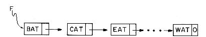
Figure 4.2 Usual Way to Draw a Linked List
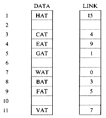
Figure 4.3a Insert GAT Into DATA(5)
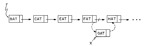
Figure 4.3b Insert Node GAT Into List
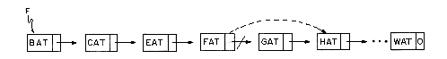
Figure 4.4 Delete GAT from List
procedure CREATE2(T)
call GETNODE(I) //get an available node//
T
 I; DATA(I) 'MAT' //store information into the node//
call GETNODE(I) //get a second available node//
LINK(T)
I // attach first node to the second//LINK(I)
0: DATA(I) 'PAT'end CREATE2
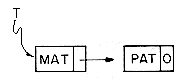
procedure INSERT(T,X)
call GETNODE(I)
DATA(I)
'OAT'if T = 0 then [T
I; LINK(I) 0] //insert into empty list//else [LINK(I)
LINK(X) //insert after X//LINK(X)
I]end INSERT
 0 is
0 is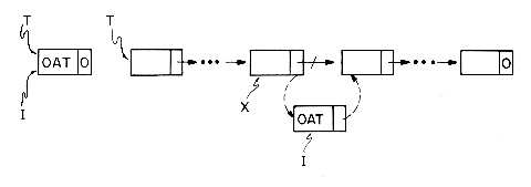
procedure DELETE(X, Y, T)
if Y= 0 then T
LINK(T) //remove the first node//else LINK(Y)
LINK(X) //remove an interiornode//
call RET(X) //return node to storage pool//
end DELETE
4.2 LINKED STACKS AND QUEUES
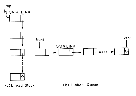
Figure 4.5
T(i) = Top of ith stack 1
 i n
i nF(i) = Front of ith queue 1
i mR(i) = Rear of ith queue 1
i mT(i) = 0 1
i nF(i) = 0 1
i mT(i) = 0 iff stack i empty
F(i) = 0 iff queue i empty
procedure ADDS(i, Y)
//add element Y onto stack i//
call GETNODE(X)
DATA(X)
Y //store data value Y into new node//LINK(X)
T(i) //attach new node to top of i-th stack//T(i)
X //reset stack pointer//end ADDS
procedure DELETES(i, Y)
//delete top node from stack i and set Y to be the DATA field of
this node//
if T(i) = 0 then call STACK__EMPTY
X
T(i) //set X to top node of stack i//Y
DATA(X) //Y gets new data//T(i)
LINK(X) //remove node from top of stack i//call RET(X) //return node to storage pool//
end DELETES
procedure ADDQ(i,Y)
//add Y to the ith queue//
call GETNODE(X)
DATA(X)
Y: LINK(X) 0if F(i) = 0 then [F(i)
R(i) X] //the queue was empty//else [LlNK(R(i))
X;R(i) X] //the queue wasnot empty//
end ADDQ
procedure DELETEQ(i, Y)
//delete the first node in the ith queue, set Y to its DATA field//
if F(i) = 0 then call QUEUE__EMPTY
else [X
F(i); F(i) LINK(X)//set X to front node//
Y
DATA(X); call RET(X)] //remove dataand return node//
end DELETEQ
4.3 THE STORAGE POOL
procedure GETNODE(I)
//I is set as a pointer to the next available node//
if AV > n then call NO__MORE__NODES
I
AVAV
AV + 1end GETNODE
procedure INIT(n)
//initialize the storage pool, through the LlNK field, to contain nodes
with addresses 1,2,3, ...,n and set AV to point to the first node
in this list//
for i
1 to n - 1 doLINK(i)
i + 1end
LlNK(n)
0AV
1end INIT
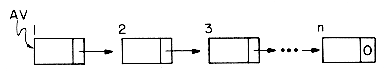
Figure 4.6 Initial Available Space List
procedure GETNODE(X)
//X is set to point to a free node if there is one on AV//
if AV = 0 then call NO__MORE__NODES
X
AVAV
LINK(AV)end GETNODE
procedure RET(X)
//X points to a node which is to be returned to the available space
list//
LINK(X)
AVAV
Xend RET
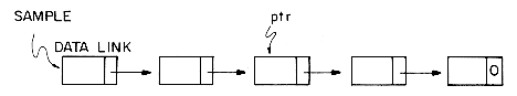 ptr + 1). These are illegal because we have no way of knowing what data was stored in what node. Therefore, we do not know what is stored either at node one or at node ptr + 1. In short, the only legal questions we can ask about a pointer variable is: 0)?
ptr
SAMPLEwhile ptr
5 doprint (DATA (ptr))
ptr
ptr + 1end
4.4 POLYNOMIAL ADDITION
_____________________
| | | |
|COEF | EXP | LINK |
|______|______|_______|
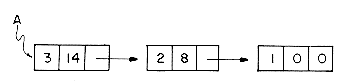
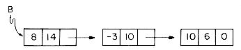
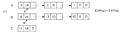
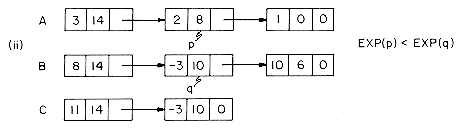
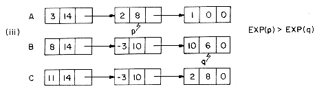
Figure 4.7 Generating the First Three Terms of C = A + B
procedure ATTACH(C,E,d)
//create a new term with COEF = C and EXP = E and attach it
to the node pointed at by d//
call GETNODE(I)
EXP(I)
ECOEF(I)
CLINK(d)
I //attach this node to the end of this list//d
I //move pointer d to the new last node//end ATTACH
procedure PADD(A,B,C)
//polynomials A and B represented as singly linked lists are
summed to form the new list named C//
1 p
A; q B //p,q pointers to next term of A, B//2 call GETNODE(C); d
C //initial node for C, returnedlater//
3 while p
0 and q 0 do //while there are more terms inA and B//
4 case
5 : EXP(p) = EXP(q): //equal exponents//
6 x
COEF(p) + COEF(q)7 if x
0 then call ATTACH(x, EXP(p),d)8 p
LINK(p); q LINK(q) //advance to nextterms//
9 : EXP(p) < EXP(q):
10 call ATTACH(COEF(q),EXP(q),d)
11 q
LINK(q) //advance to next term//12 : else: call ATTACH(COEF(p),EXP(p),d)
13 p
LINK(p) //advance to next term of A//14 end
15 end
16 while p
0 do //copy remaining terms of A//17 call ATTACH(COEF(p),EXP(p),d)
18 p
LINK(p)19 end
20 while q
0 do //copy remaining terms of B//21 call ATTACH(COEF(q),EXP(q),d)
22 q
LINK(q)23 end
24 LINK(d)
0; t C; C LINK(C) //delete extra initialnode//
25 call RET(t)
26 end PADD
0 and em > ... > e1  0, fn > ... > f1 0. coefficient additions min {m, n}.
call READ(A)
call READ(B)
call READ(C)
T
PMUL(A, B)D
PADD(T, C)call PRINT(D)
procedure ERASE(T)
//return all the nodes of T to the available space list avoiding repeated
calls to procedure RET//
if T = 0 then return
p
Twhile LINK (p)
0 do //find the end of T//p
LINK (p)end
LlNK (p)
AV // p points to the last node of T//AV
T //available list now includes T//end ERASE
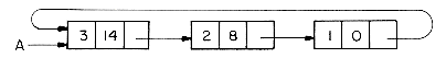
Figure 4.8 Circular List Representation of A = 3x14 + 2x8 + 1
procedure CERASE(T)
//return the circular list T to the available pool//
if T = 0 then return;
X
LINK (T)LINK(T)
AVAV
Xend CERASE

Figure 4.9 Dashes Indicate Changes Involved in Erasing a Circular List
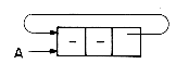
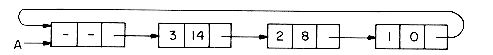 LINK (A); q LINK(B)A and q B do A do B do C EXP(q) the remaining terms of B can be copied by further executions of the case statement. The same is true if all nodes of B are examined before those of A This implies that there is no need for additional code to copy the remaining terms as in PADD. The final algorithm takes the following simple form.
procedure CPADD (A, B, C)
//polynomials A and B are represented as circular lists with head
nodes so that EXP(A) = EXP(B) = -1. C is returned as their sum,
represented as a circular list//
p
LINK (A); q LINK(B)call GETNODE(C); EXP(C)
-1 //set up head node//d
C //last node in C//loop
case
: EXP(p) = EXP(q): if EXP(p)=-1then [LINK(d)
C; return]x
COEF(p) + COEF(q)if x
0 then call ATTACH(x,EXP(p),dp
LINK(p); q LINK(q): EXP(p) < EXP(q): call ATTACH(COEF(q), EXP(q),d)
q
LINK(q): else : call ATTACH(COEF(p), EXP(p),d)
p
LINK(p)end
forever
end CPADD
4.5 MORE ON LINKED LISTS
procedure INVERT(X)
//a chain pointed at by X is inverted so that if X = (a1, ...,am)
then after execution X = (am, ...,a1)//
p
X;q 0while p
0 dor
q;q p //r follows q; q follows p//p
LINK(p) //p moves to next node//LINK(q)
r //link q to previous node//end
X
qend INVERT
1 nodes, the while loop is executed m times and so the computing time is linear or O(m).procedure CONCATENATE(X, Y, Z)
//X = (a1, ...,am), Y = (b1, ...,bn), m,n
0, produces a new chainZ = (a1, ...,am,b1 , ...,bn)//
Z
Xif X = 0 then [Z
Y; return]if Y = 0 then return
p
Xwhile LINK(p)
0 do //find last node of X//p
LINK(p)end
LINK(p)
Y //link last node of X to Y//end CONCATENATE
procedure CONCATENATE(X, Y, Z)
case
: X = 0 :Z
Y: Y = 0 : Z
X: else : p
X; Z Xwhile LINK(p)
0 dop
LINK (p)end
LINK(p)
Yend
end CONCATENATE
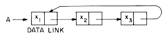
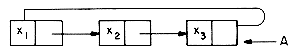
procedure INSERT__FRONT(A, X)
//insert the node pointed at by X to the front of the circular list
A, where A points to the last node//
if A = 0 then [A
XLINK (X)
A]else [LINK(X)
LINK (A)LINK(A)
X]end INSERT--FRONT
X to the else clause of INSERT_-_FRONT.procedure LENGTH(A)
//find the length of the circular list A//
i
0if A
0 then [ptr Arepeat
i
i + 1; ptr LINK(ptr)until ptr = A ]
return (i)
end LENGTH
4.6 EQUIVALENCE RELATIONS
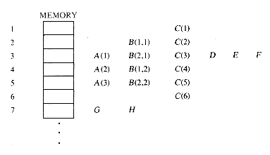
 and suppose that: x, e.g. x is to be assigned the same location as itself. Thus is reflexive. y then y x, e.g. assigning y the same location as x is the same as assigning x the same location as y. Thus, the relation is symmetric. y and y z then x z, e.g. if x and y are to be assigned the same location and y and z are also to be assigned the same location, then so also are x and z. The relation is transitive., over a set S, is said to be an equivalence relation over S iff it is symmetric, reflexive and transitive over S. y. For example, if we have 12 variables numbered 1 through 12 and the following equivalences were defined via the EQUIVALENCE statement:
1
5, 4 2, 7 11, 9 10, 8 5, 7 9, 4 6, 3 12 and 12 1procedure EQUIVALENCE (m,n)
initialize
for k
1 to m doread the next pair (i,j)
process this pair
end
initialize for output
repeat
output a new equivalence class
until done
end EQUIVALENCE
procedure EQUIVALENCE (m,n)
declare SEQ(1:n), DATA(1:2m), LINK(1:2m), BIT(1:n)
initialize BIT, SEQ to zero
for k
1 to m doread the next pair (i,j)
put j on the SEQ(i) list
put i on the SEQ(j) list
end
index
1repeat
if BIT(index) = 0
then [BIT(index)
1output this new equivalence class]
index
index + 1until index > n
end
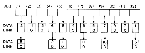 j, two nodes are used. SEQ(i) points to a list of nodes which contains every number which is directly equivalenced to i by an input relation. i n such that BIT(i) = 0. Each element in the list SEQ(i) is printed. In order to process the remaining lists which, by transitivity, belong in the same class as i a stack of their nodes is created. This is accomplished by changing the LINK fields so they point in the reverse direction. The complete algorithm is now given.
procedure EQUIVALENCE (m,n)
//Input: m, the number of equivalence pairs
n, the number of variables
Output: variables 1, ...,n printed in equivalence classes//
declare SEQ(1:n), BIT(1:n)
DATA(1: 2m), LINK(1: 2m);
for i
1 to n do SEQ(i) BIT(i) 0 endav
1for k
1 to m do //phase 1: process all input//read next equivalence pair (i, j)
DATA(av)
j; LlNK(av) SEQ(i) //add j to list i//SEQ(i)
av; av av + 1DATA(av)
i; LINK(av) SEQ(j) //add i to list j//SEQ(j)
av; av av + 1end
index
1repeat //phase 2: output all classes//
if BIT (index) = 0
then [print ('A new class', index)BIT(index)
1 //mark class as output//ptr
SEQ(index); top 0 //initialize stack//loop //find the entire class//
while ptr
0 do //process a list//j
DATA (ptr)if BIT(j) = 0
then [print (j); BIT(j)
1t
LINK (ptr); LINK (ptr) toptop
ptr; ptr t]else ptr
LINK (ptr)end
if top = 0 then exit //stack empty//
ptr
SEQ(DATA(top))top
LINK (top)forever]
index
index + 1until index > n
end EQUIVALENCE
Analysis of Algorithm EQUIVALENCE
4.7 SPARSE MATRICES
0, then there will be a node with VALUE field aij, ROW field i and COL field j. This node will be linked into the circular linked list for row i and also into the circular linked list for column j. It will, therefore, be a member of two lists at the same time .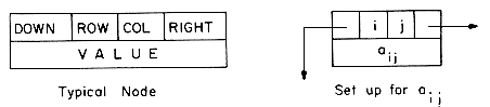
Figure 4.10 Node Structure for Sparse Matrix Representation

Figure 4.11 6 x 7 Sparse Matrix A
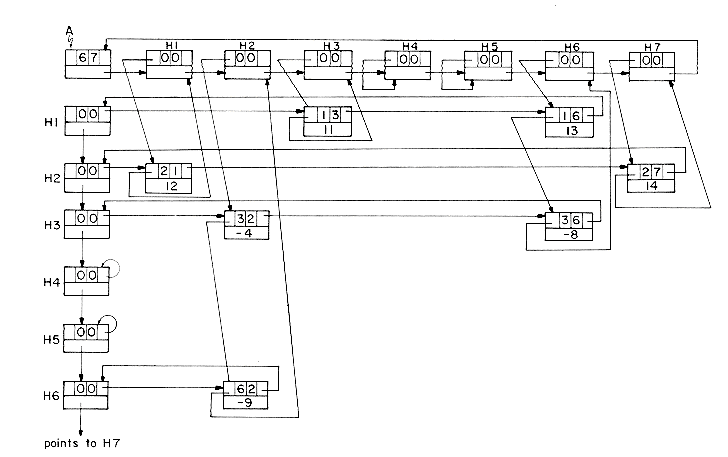
Figure 4.12 Linked Representation of the Sparse Matrix A
Analysis of Algorithm MREAD
procedure MERASE(A)
//return all nodes of A to available space list. Assume that the available
space list is a singly linked list linked through the field RIGHT
with AV pointing to the first node in this list.//
RIGHT(A)
AV; AV A; NEXT VALUE(A)while NEXT
A do //erase circular lists by rows//T
RIGHT(NEXT)RIGHT(NEXT)
AVAV
TNEXT
VALUE(NEXT)end
end MERASE
Analysis of Algorithm MERASE
procedure MREAD(A)
//read in a matrix A and set up its internal representation as
discussed previously. The triples representing nonzero terms
are assumed ordered by rows and within rows by columns.
An auxiliary array HDNODE is used.//
1 read (n,m,r) //m, n are assumed positive. r is the number
of nonzero elements//
2 p
max {m,n}3 for i
1 to p do //get p headnodes for rows andcolumns//
4 call GETNODE(X); HDNODE(i)
X5 ROW(X)
COL(X) 06 RIGHT(X)
VALUE(X) X //these fields point tothemselves//
7 end
8 current_row
1; LAST HDNODE(1)9 for i
1 to r do10 read (rrow, ccol, val) //get next triple//
11 if rrow > current__row //current row is done; close it and
begin another//
12 then [RIGHT(LAST)
HDNODE(current__row)13 current__row
rrow; LAST HDNODE(rrow)]//LAST points to rightmost node//
14 call GETNODE(X)
15 ROW(X)
rrow; COL(X) ccol; VALUE(X) val//store triple into new node//
16 RIGHT(LAST)
X; LAST X //link into row list//17 DOWN(VALUE(HDNODE(ccol)))
X;//link into column list//
18 VALUE(HDNODE(ccol))
X19
20 end
21 //close last row//
if r
0 then RIGHT(LAST) HDNODE(current__row)22 for i
1 to m do //close all column lists//23 DOWN(VALUE(HDNODE(i))) HDNODE(i)
24 end
25 //set up list of headnodes linked through VALUE field//
26 call GETNODE(A): ROW(A)
n; COL(A) m//set up headnode of matrix//
27 for i
1 to p - 1 do VALUE(HDNODE(i)) HDNODE(i + 1)end
28 if p = 0 then VALUE(A)
A29 else [VALUE(HDNODE(p))
AVALUE(A)
HDNODE(1)]30 end MREAD
4.8 DOUBLY LINKED LISTS AND DYNAMIC STORAGE MANAGEMENT
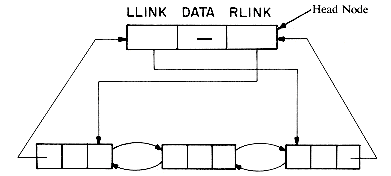
Figure 4.13 Doubly Linked Circular List with Head Node
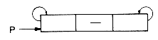
procedure DDLETE(X, L)
if X = L then call NO__MORE__NODES
//L is a list with at least one node//
RLINK(LLINK(X))
RLINK(X)LLINK(RLINK(X))
LLINK(X)call RET(X)
end DDLETE

procedure DINSERT (P, X)
//insert node P to the right of node X//
LLINK(P)
X //set LLINK and RLINK fields of node P//RLINK(P)
RLINK(X)LLINK(RLINK(X))
PRLINK(X)
Pend DINSERT
Dynamic Storage Management
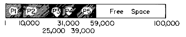
Figure 4.14 Memory After Allocation to P1-P5
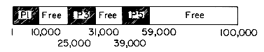
Figure 4.15 Status of Memory After Completion of P2 and P4
N and allocating N words out of this block. Such an allocation strategy is called first fit. The algorithm below makes storage allocations using the first fit strategy. An alternate strategy, best fit, calls for finding a free block whose size is as close to N as possible, but not less than N. This strategy is examined in the exercises.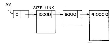
Figure 4.16 Free List with Head Node Corresponding to figure 4.15
procedure FF(n, p)
//AV points to the available space list which is searched for a node
of size at least n. p is set to the address of a block of size n
that may be allocated. If there is no block of that size then p = 0.
It is assumed that the free list has a head node with SIZE field = 0//
p
LINK(AV); q AVwhile p
0 doif SIZE(p)
n then [SIZE(p) SIZE(p) - nif SIZE(p) = 0 then LINK(q)
LINK(p)else p
p + SIZE(p)return]
q
p; p LINK (p)end
//no block is large enough//
end FF
 such that if the allocation of a portion of a node leaves behind a node of size <, then the entire node is allocated. I.e., we allocate more storage than requested in this case. The second problem arises from the fact that the search for a large enough node always begins at the front of the list. As a result of this, all the small nodes tend to collect at the front so that it is necessary to examine several nodes before an allocation for larger blocks can be made. In order to distribute small nodes evenly along the list, one can begin searching for a new node from a different point in the list each time a request is made. To implement this. the available space list is maintained as a circular list with a head node of size zero. AV now points to the last node from which an allocation was made. We shall see what the new allocation algorithm looks like after we discuss what has to be done to free a block of storage.
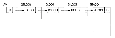
Figure 4.17 Available Space List When Adjacent Free Blocks Are Not Coalesced.
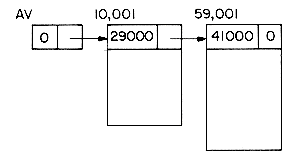
Figure 4.18 Available Space List When Adjacent Free Blocks Are Coalesced.
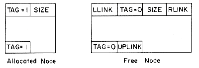
Figure 4.19

procedure ALLOCATE (n,p)
//Use next fit to allocate a block of memory of size at least
n, n > 0. The available space list is maintained as described
above and it is assumed that no blocks of size <
are tobe retained. p is set to be the address of the first word in
the block allocated. AV points to a node on the available list.//
1 p
RLINK(AV) //begin search at p//2 repeat
3 if SIZE (p)
n then //block is big enough//4 [diff
SlZE(p) - n5 if diff <
then //allocate whole block//6 [RLINK (LLINK(p))
RLINK(p) //delete nodefrom AV//
7 LLINK(RLlNK(p))
LLINK(p)8 TAG(p)
TAG(p + SlZE(p) - 1) 1 //settags//
9 AV
LLINK(p) //set starting point of nextsearch//
10 return]
11 else //allocate lower n words//
12 [SIZE(p)
diff13 UPLINK (p + diff - 1)
p14 TAG(p + diff - 1)
0 //set upper portion asunused//
15 AV
p //position for next search//16 p
p + diff //set p to point to start of allocatedblock//
17 SlZE(p)
n18 TAG(p)
TAG(p + n - 1) 1//set tags for allocated block//
19 return]]
20 p
RLlNK(p) //examine next node on list//21 until p = RLINK(AV)
22 //no block large enough//
23 p
0;24 end ALLOCATE
procedure FREE(p)
//return a block beginning at p and of size SlZE(p)//
1 n
SlZE(p)2 case
3 :TAG(p - 1) = 1 and TAG(p + n) = 1:
//both adjacent blocks in use//
4 TAG(p)
TAG(p + n - 1) 0 //set up a freeblock//
5 UPLINK (p + n - 1)
p6 LLINK(p)
AV; RLINK (p) RLINK (AV)//insert at right of AV//
7 LLINK (RLlNK(p))
p; RLINK(AV) p8 :TAG(p + n) = 1 and TAG(p - 1) = 0: //only left block
free//
9 q
UPLINK (p - 1 ) //start of left block//10 SIZE(q)
SlZE(q) + n11 UPLINK(p + n - 1)
q; TAG(p + n - 1) 012 :TAG(p + n) = 0 and TAG(p - 1) = 1:
//only right adjacent block free//
13 RLINK(LLINK(p + n))
p //replace blockbeginning//
14 LLINK(RLINK(p + n))
p //at p + n by one//15 LLINK(p)
LLINK(p + n) //beginning at p//16 RLINK(p)
RLINK(p + n)17 SlZE(p)
n + SlZE(p + n)18 UPLINK(p + SIZE(p) - 1)
p19 TAG(p)
020 AV
p21 :else: //both adjacent blocks free//
22 //delete right free block from AV list//
RLINK (LLINK(p + n))
RLINK (p + n)23 LLINK(RLINK(p + n))LLINK(p + n)
24 q
UPLINK(p - 1) //start of left freeblock//
25 SIZE(q)
SIZE(q) + n + SIZE(p + n)26 UPLINK(q + SIZE(q) - 1)
q27 AV
LLINK(p + n)28 end
29 end FREE
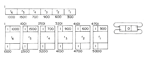
Figure 4.20
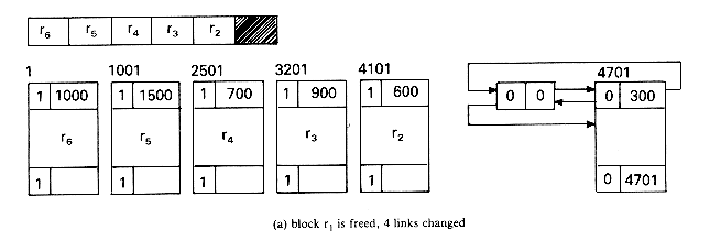
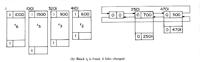
Figure 4.21 Freeing of Blocks in Boundary Tag System
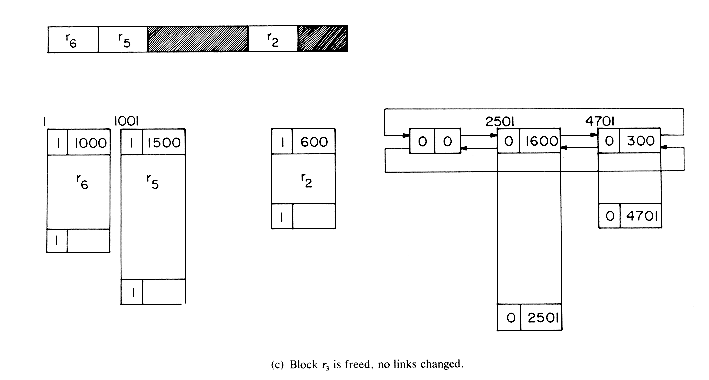
Figure 4.21 Freeing of Blocks in Boundary Tag System (contd.)
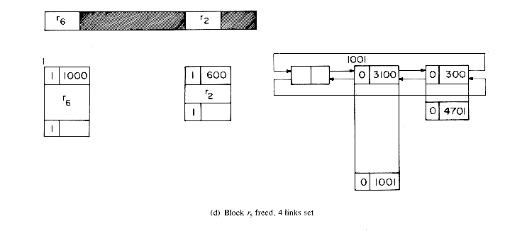
Figure 4.21 Freeing of Blocks in Boundary Tag System (contd.)
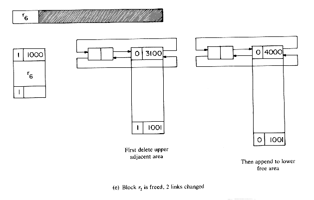
Figure 4.21 Freeing of Blocks in Boundary Tag System (contd.)
4.9 GENERALIZED LISTS
0 elements,  1,...,n, which we write as A = (1, ...,n). The elements of a linear list are restricted to be atoms and thus the only structural property a linear list has is the one of position, i.e. i precedes i+1, 1 i < n. It is sometimes useful to relax this restriction on the elements of a list, permitting them to have a structure of their own. This leads to the notion of a generalized list in which the elements i, 1 i n may be either atoms or lists.1, ..., nwhere the i are either atoms or lists. The elements i, 1 i n which are not atoms are said to be the sublists of A.1, ..., n). A is the name of the list (1, ..., n) and n its length. By convention, all list names will be represented by capital letters. Lower case letters will be used to represent atoms. If n 1, then 1 is the head of A while (2, ..., 2) is the tail of A.
(i) D = ( ) the null or empty list, its length is zero.
(ii) A = (a, (b,c)) a list of length two; its first element is
the atom 'a' and its second element is the
linear list (b,c).
(iii) B = (A,A,( )) a list of length three whose first two
elements are the lists A, the third element
the null list.
(iv) C = (a, C) a recursive list of length two. C corresponds
to the infinite list C = (a,(a,(a, ...).

Figure 4.22 Representation of P(x,y,z) using three fields per node
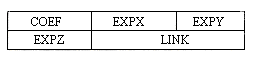
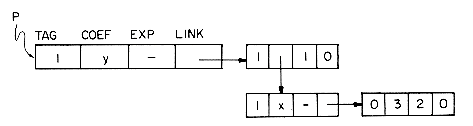
________________________
| | | |
|TAG = 0/1 | DATA | LINK |
|__________|______|______|
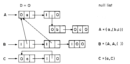
Figure 4.23 Representation of Lists i-iv
Recursive Algorithms for Lists
procedure COPY (L)
//L points to a nonrecursive list with no common sublists. COPY
returns a pointer to a new list which is a duplicate of L//
ptr
0if L
0 then[if TAG(L) = 0 then q
DATA(L) //save an atom//else q
COPY(DATA(L)) //recursion//r
COPY(LINK(L)) //copy tail//call GETNODE(ptr) //get a node//
DATA(ptr)
q; LINK(ptr) r //combine head and tail//TAG(ptr)
TAG(L)]return (ptr)
end COPY
procedure COPY(L)
//nonrecursive version//
i
0 //initialize stack index//1: ptr
0if L
0 then[if TAG(L) = 0
then q
DATA(L)else [STACK(i + 1)
q //stack local variables//STACK(i + 2)
rSTACK(i + 3)
ptrSTACK(i + 4)
L //stack parameter//STACK(i + 5)
2 //stack return address//i
i + 5;L
DATA(L); go to 1 //set parameter andbegin//
2: q
STACK(i) //remove function value//i
i - 1]STACK(i + 1)
q; STACK(i + 2) r //stackvariables and//
STACK(i + 3)
ptr; STACK(i + 4) L//parameter for second//
STACK(i + 5)
3; i i +5 //recursive call//L
LINK(L); go to 13: r
STACK(i); i i 1 //remove function value//call GETNODE(ptr)
DATA(ptr)
q; LlNK(ptr) rTAG(ptr)
TAG(L)]if i
0 then [addr STACK(i); L STACK(i - 1)//execute a return//
t
STACK(i - 2); r STACK(i - 3)q
STACK(i - 4);STACK(i - 4)
ptr; ptr t //store functionvalue//
i
i - 4; go to addr] //branch to 2 or 3//return (ptr)
end COPY
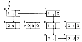
Figure 4.24 Linked Representation for A
Levels of Continuing Continuing
recursion Value of L Levels L Levels L
1 q 2 r 3 u
2 s 3 u 4 v
3 t 4 w 5 o
4 o 5 x 4 v
3 t 6 o 3 u
2 s 5 x 2 r
1 q 4 w 3 o
2 r
1 q
Figure 4.25 Values of Parameter in Execution of COPY(A)
procedure EQUAL(S,T)
//S and T are nonrecursive lists, each node having three fields: TAG,
DATA and LINK. The procedure returns the value true if the
lists are identical else false//
ans
falsecase
:S = 0 and T = 0: ans
true:S
0 and T 0:if TAG(S) = TAG(T)
then [if TAG(S) = 0
then ans
DATA (S) = DATA(T)else ans
EQUAL(DATA(S),DATA(T))if ans then
ans
EQUAL(LINK(S),LINK(T))]end
return (ans)
end EQUAL
procedure DEPTH(S)
//S is a nonrecursive list having nodes with fields TAG, DATA an
LINK. The procedure returns the depth of the list//
max
0if S = 0 then return (max) //null list has zero depth//
ptr
Swhile ptr
0 doif TAG(ptr) = 0 then ans
0else ans
DEPTH(DATA(ptr)) //recursion//if ans > max then max
ans //find a new maximum//ptr
LINK(ptr)end
return (max + 1)
end DEPTH
Reference Counts, Shared and Recursive Lists
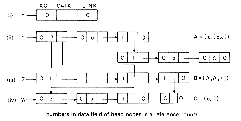
Figure 4.26 Structure with Head Nodes for Lists i-iv
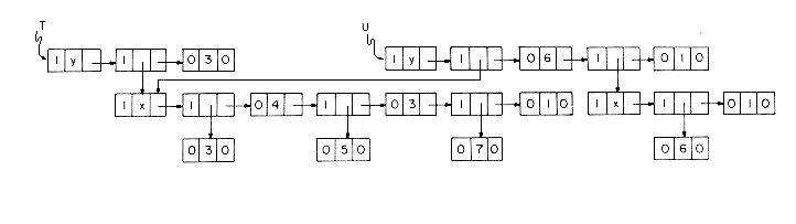
Figure 4.27 T = (3x4 + 5x3 + 7x)y3 U = (3x4 + 5x3 + 7x)y6 + 6xy
procedure LERASE(X)
//recursive algorithm to erase a list assuming a REF field in each
head node which has the number of pointers to this list and a
TAG field such that TAG(X) = 0 if DATA(X) is actually an atom
and TAG(X) = 1 if DATA(X) is a link to a sublist. The storage
pool is assumed linked through the field LINK with AV pointing
to the first node in the pool//
REF(X)
REF(X) - 1 //decrement reference count//if REF(X)
0 then returnY
X // Y will traverse top level of X//while LINK(Y)
0 doY
LINK(Y)if TAG(Y) = 1 then call LERASE (DATA (Y))// recursion//
end
LINK(Y)
AV //attach top level nodes to avail list//AV
Xend LERASE

Figure 4.28 Indirect Recursion of Lists A and B Pointed to by Program Variables R and S.
4.10 GARBAGE COLLECTION AND COMPACTION
Marking
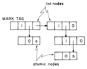
procedure DRIVER
//driver for marking algorithm. n is the number of nodes in the
system//
1 for i
1 to n do //unmark all nodes//2 MARK (i)
03 end
4 MARK (0)
1; TAG (0) 0 //boundary conditions//5 for each pointer variable X with MARK (X) = 0 do
6 MARK (X)
17 if TAG(X) = 1 then call MARK1(X) //X is a list node//
8 end
9 end DRIVER
Analysis of MARK1
procedure MARK1 (X)
//X is a list node. Mark all nodes accessible from X. It is assumed
that MARK(0) = 1 and TAG(0) = 0. ADD and DELETE
perform the standard stack operations//
1 P
X; initialize stack2 loop //follow all paths from P, P is a marked list node//
3 loop //move downwards stacking RLINK's if needed//
4 Q
RLINK (P)5 if TAG(Q) = 1 and MARK(Q) = 0 then call ADD(Q)
//stack Q//
6 MARK(Q)
1 //Q may be atomic//7 P
DLINK (P)//any unmarked nodes accessible from P?//
8 if MARK(P) = 1 or TAG(P) = 0 then exit
9 MARK(P)
110 forever
11 MARK(P)
1 //P may be an unmarked atomic node//12 if stack empty then return //all accessible nodes marked//
13 call DELETE(P) //unstack P//
14 forever
15 end MARK1
q = p - r. Also, the number of iterations of the loop of lines 2-14 is one plus the number of nodes that get stacked. The only nodes that can be stacked are those previously unmarked (line 5). Once a node is stacked it gets marked (line 6). Hence r m + 1. From this and the knowledge that m p - r, we conclude that p 2m + 1. The computing time of the algorithm is O(p + r). Substituting for p and r we obtain O(m) as the computing time. The time is linear in the number of new nodes marked! Since any algorithm to mark nodes must spend at least one unit of time on each new node marked, it follows that there is no algorithm with a time less than O(m). Hence MARK1 is optimal to within a constant factor (recall that 2m = O (m) and 10m = O(m)).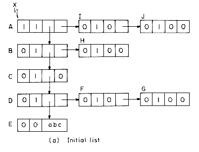
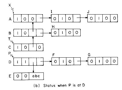
Figure 4.29 Example List for MARK2
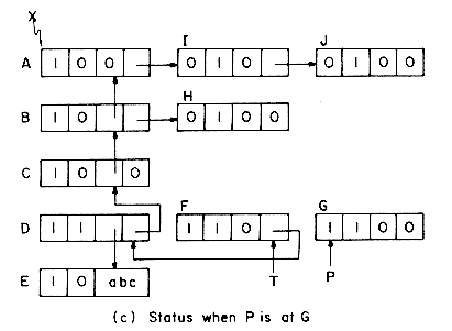
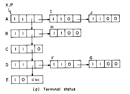
A B C D F G F D C B H B A I J I A
(e) Path taken by P
Figure 4.29 Example List for MARK2 (contd.)
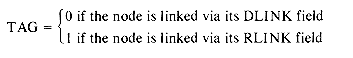
procedure MARK 2(X)
//same function as MARK1//
//it is assumed that MARK(0) = 1 and TAG(0) = 0//
1 P
X; T 0 //initialize T - X path list//2 repeat
3 Q
DLINK(P) //go down list//4 case
5 :MARK(Q) = 0 and TAG(Q) = 1: //Q is an unexamined
list node//
6 MARK(Q)
1; TAG(P) 07 DLINK(P)
T; T P //add Pto T - X path list//8 P
Q //move down to explore Q//9 :else: //Q is an atom or already examined//
10 MARK(Q)
111 L1: Q
RLINK(P) //move right of P//12 case
13 :MARK(Q) = 0 and TAG(Q) = 1: //explore Q
further//
14 MARK(Q)
115 RLINK (P)
T; T P16 P
Q17 :else: MARK(Q)
1 //Q is not to be explored;back up on path list//
18 while T
0 do //while path list not empty//19 Q
T20 if TAG(Q) = 0 //link to P through DLINK//
21 then [T < DLINK(Q); DLINK (Q)
P22 TAG(Q)
1; P Q; go to L1]//P is node to right of Q//
23 T
RLINK(Q); RLINK(Q) P24 P
Q25 end
26 end
27 end
28 until T= 0
29 end MARK 2
Analysis of MARK2
Storage Compaction
i 8 being the size of the ith node.
Figure 4.30 Memory Configuration After Marking. Free Nodes Have MARK bit = O

Figure 4.31 Available Space List Corresponding to Figure 4.30
Figure 4.32 Memory Configuration After Reallocating Storage to Nodes in Use

Figure 4.33
procedure COMPACT(MEMORY, MARK,SlZE, M, NEW__ADDR)
//compact storage following the marking phase of garbage collection.
Nodes in use have MARK bit=1. SlZE(i)= number of words
in that node. NEW__ADDR is a free field in each node. Memory
is addressed 1 to M and is an array MEMORY.//
//phase I: Scan memory from left assigning new addresses to nodes
in use. AV = next available word//
AV
1;i 1 //variable i will scan all nodes left to right//while i
M doif MARK(i) = 1 then [//relocate node//
NEW__ADDR(i)
AVAV
AV + SIZE(i)]i
i + SIZE(i) //next node//end
//phase II: update all links. Assume the existence of a fictitious
node with address zero and NEW__ADDR(0) = 0//
i
1while i
M doif MARK(i) = 1 then [//update all links to reflect new
addresses//
LINK1(i)
NEW_ADDR(LINK1(i))LlNK2(i)
NEW_ADDR(LINK2(i))]i
i + SIZE(i)end
//phase III: relocate nodes//
i
1while i
M doif MARK (i) = 1 then [//relocate to NEW_ADDR(i)//
k
NEW_ADDR(i); l kfor j
i to i + SIZE(i) - 1 doMEMORY(k)
MEMORY(j)k
k+ 1end
i
i + SIZE(l)]else i
i + SIZE(i)end
end COMPACT
 size of nodes relocated)). In the case of generalized lists, garbage collection is necessitated by the absence of any other efficient means to free storage when needed. Garbage collection has found use in some programming languages where it is desirable to free the user from the task of returning storage. In both situations, a disciplined use of pointer variables and link fields is required. Clever coding tricks involving illegal use of link fields could result in chaos during marking and compaction. While compaction has been presented here primarily for use with generalized list systems using nodes of variable size, compaction can also be used in other environments such as the dynamic storage allocation environment of section 4.8. Even though coalescing of adjacent free blocks takes place in algorithm FREE of section 4.8, it is still possible to have several small nonadjacent blocks of memory free. The total size of these blocks may be large enough to meet a request and it may then be desirable to compact storage. The compaction algorithm in this case is simpler than the one described here. Since all addresses used within a block will be relative to the starting address rather than the absolute address, no updating of links within a block is required. Phases I and III can, therefore, be combined into one phase and phase II eliminated altogether. Since compaction is very slow one would like to minimize the number of times it is carried out. With the introduction of compaction, several alternative schemes for dynamic storage management become viable. The exercises explore some of these alternatives.
4.11 STRINGS--A CASE STUDY
structure STRING
declare NULL( )
 string; ISNULL (string) boolean
IN (string, char)
string; LEN (string) integerCONCAT (string, string)
stringSUBSTR (string, integer, integer)
stringLINK_DEST 3184string, string)
integer;for all S,T
string, i,j integer, c,d char letISNULL (NULL) :: = true; ISNULL (IN(S,c)) :: = false
LEN (NULL) :: = 0; LEN (IN(S,c)) :: = 1 + LEN(S)
CONCAT (S,NULL):: = S
CONCAT (S,IN(T,c)) :: = IN (CONCAT (S,T),c)
SUBSTR (NULL,i,j):: = NULL
SUBSTR (IN(S,c),i,j) :: =
if j = 0 or i + j - 1 > LEN(IN(S,c)) then NULL
else if i + j - 1 = LEN(IN(S,c))
then IN(SUBSTR (S,i,j - 1 ),c)
else SUBSTR(S,i,j)
INDEX (S,NULL) :: = LEN (S) + 1
INDEX (NULL,IN(T,d)) :: = 0
INDEX (IN(S,c),IN(T,d)) :: =
if c = d and INDEX(S,T) = LEN(S) - LEN(T) + 1
then INDEX(S,T) else INDEX(S,IN(T,d))
end
end STRING
SUBSTR(S,2,1) = SUBSTR(IN(IN(IN(NULL,a),b),c),2,1)
= SUBSTR(IN(IN(NULL,a),b),2,1)
= IN(SUBSTR(IN(NULL,a),2,0),b)
= IN(NULL,b)
= 'b'
= IN(SUBSTR(IN(IN(IN(NULL,a),b),c),3,1),d)
= IN(IN(SUBSTR(IN(IN(NULL,a),b),3,0),c),d)
= IN(IN(NULL,c),d)
= 'cd'
4.11.1 DATA REPRESENTATIONS FOR STRINGS
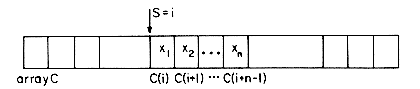
Figure 4.34 Sequential Representation of S = 'x1 ... xn'
 or by compacting the space originally occupied by this substring (figure 4.36). The former entails storage waste while the latter in the worst case takes time proportional to LENGTH(S). The replacement of a substring of S by another string T is efficient only if the length of the substring being replaced is equal to LENGTH(T). If this is not the case, then some form of string movement will be required.
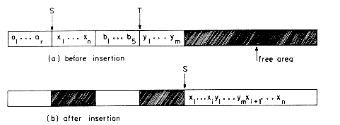
Figure 4.35 Insertion Into a Sequential String
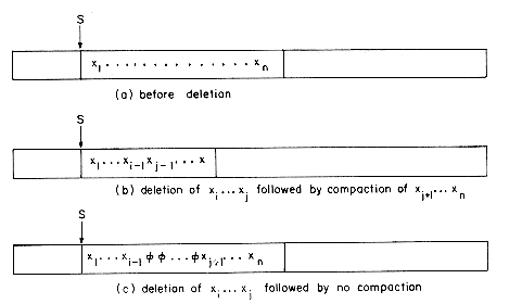
Figure 4.36 Deletion of a Substring
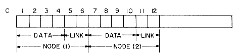
Figure 4.37 Partitioning Available Memory Into Nodes of Size 4.
(figure 4.38(a) ). An in place insertion might require one node to be split into two as in figure 4.38(b). Deletion of a substring can be carried out by replacing all characters in this substring by and freeing nodes in which the DATA field consists only of 's. In place replacement can be carried similarly. Storage management is very similar to that of section 4.3. Storage compaction may be carried out when there are no free nodes. Strings containing many occurrences of could be compacted freeing several nodes. String representation with variable sized nodes is similar.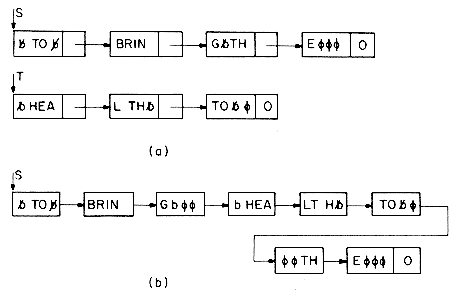
Figure 4.38
procedure SINSERT(S,T,i)
//insert string T after the i-th character of S destroying the original//
//strings S,T and creating a new string S//
1 case //degenerate cases//
2 :i < 0 or i > LENGTH(S): print ('string length error'); stop3 : T = 0: return
4 : S = 0: S
T; return5 end
//at this point LENGTH(S) > 0, LENGTH(T) > 0, 0
i LENGTH(S)//
6 ptr
S; j 17 while j < i do //find i-th character of S//
8 ptr
LINK (ptr); j j + 1 //ptr points to i-th node//9 end
10 if i = 0 then [save
S; ptr T; S T] //save i + 1 character//11 else [save
LINK (ptr)12 LINK (ptr)
T] //attach list T to list S//13 while LINK (ptr)
0 do //find end of T//14 ptr
LINK (ptr)15 end
16 LINK (ptr)
save //point end of T to////i + 1-st character of S//
17 end SINSERT
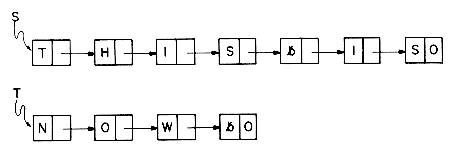
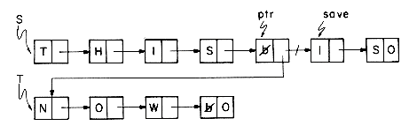

Figure 4.39 Circular Representation of S and T
ptr S; j
0while j < i do
ptr
LINK (ptr); j j + 1 //find i-th character of S//end
save
LINK (ptr) //save i + 1-st character of S//else LINK (ptr)
LINK (T)LINK (T)
save //attach end of T to S//if ptr = S and i
0 then S T4.11.2 PATTERN MATCHING IN STRINGS
procedure FIND (S,PAT,i)
//find in string S the first occurrence of the string PAT and return
i as a pointer to the node in S where PAT begins. Otherwise return
i as zero//
i
0if PAT = 0 or S = 0 then return
p
Srepeat
save
p; q PAT //save the starting position//while p
0 and q 0 and DATA(p) = DATA(q) dop
LINK (p); q LINK (q) //characters match,move to next pair//
end
if q = 0 then [i
save; return] //a match is found//p
LINK (save) //start at next character in S//until p = 0 //loop until no more elements in S//
end FIND
procedure NFIND (S,PAT,i)
//string S is searched for PAT and i is set to the first node in S
where PAT occurs else zero. Initially the last and first characters
of PAT are checked for in S//
i
0if PAT = 0 or S = 0 then return
p
q PAT;t 0while LINK (q)
0 do //q points to last node of PAT//q
LINK(q); t t + 1end //t + 1 is the length of PAT//
j
r save Sfor k
1 to t while j 0 do //find t + 1-st node of S//j
LINK (j)end
while j
0 do //while S has more chars to inspect//p
PAT; r saveif DATA(q) = DATA(j) //check last characters//
then [while DATA(p) = DATA(r) and p
q dop
LINK(p); r LINK(r) //check pattern//end
if p = q then [i
save; return]] //success//save
LINK (save); j LINK(j)end
end NFIND
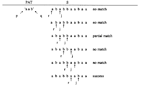
Figure 4.40 Action of NFIND on S and PAT
PAT = 'a b c a b c a c a b'
a then clearly, we may proceed by comparing si + 1 and a. Similarly if si = a and si+1 b then we may proceed by comparing si+1 and a. If si si+1 = ab and si+2 c then we have the situation:S = ' - a b ? ? ? . . . . ?'
PAT = ' a b c a b c a c a b'
c. At this point we know that we may continue the search for a match by comparing the first character in PAT with si+2. There is no need to compare this character of PAT with si + l as we already know that si + 1 is the same as the second character of PAT, b and so si + 1 a. Let us try this again assuming a match of the first four characters in PAT followed by a non-match i.e. si+4 b. We now have the situation:S = ' - a b c a ? ? . . . ?'
PAT = ' a b c a b c a c a b'
j 1 2 3 4 5 6 7 8 9 10
PAT a b c a b c a c a b
f 0 0 0 1 2 3 4 0 1 2
pj then matching may be resumed by comparing si and Pf(j-1)+1 If j 1. If j = 1, then we may continue by comparing si+1 and p1. j n, then we define
Figure 4.41 shows the pattern PAT with the NEXT field included.
procedure PMATCH (S,PAT)
//determine if PAT is a substring of S//
1 i
S //i will move through S//2 j
PAT //j will move through PAT//3 while i
0 and j 0 do4 if DATA (i) = DATA (j)
5 then [//match//
6 i
LINK (i)7 j
LINK (j)]8 else [if j = PAT then i
LINK(i)9 else j
NEXT(j]10 end
11 if j = 0 then print ('a match')12 else print ('no match')13 end PMATCH
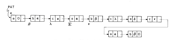
Figure 4.41 Augmented Pattern PAT with NEXT Field
procedure FAIL (PAT,f)
//compute the failure function for PAT = p1p2 ... pn//
1 f(1)
02 for j
2 to n do //compute f(j)//3 i
f(j - 1)4 while pj
pi + 1 and i > 0 do5 i
f(i)6 end
7 if pj = pi + 1 then f(j)
i + 18 else f(j)
09 end
10 end FAIL
4.12 IMPLEMENTING NODE STRUCTURES
i 200 can be determined or changed through the use of standard assignment statements. With this structure for nodes, the following FORTRAN subroutine would perform the function of algorithm INIT of section 4.3. SUBROUTINE INIT(N)
C LINK N NODES TO FORM THE INITIAL AVAILABLE
C SPACE LIST AND SET AV TO POINT TO FIRST NODE.
C ARRAYS EXP, COEF AND LINK AND VARIABLE AV
C ARE IN BLANK COMMON.
INTEGER EXP(200),COEF(200),LINK(200),AV
COMMON EXP,COEF,LINK,AV
M = N - 1
DO 10 I = 1, M
10 LINK(I) = I + 1
LINK(N) = 0
AV= 1
RETURN
END
PROCEDURE INIT(N: INTEGER);
{This procedure initializes the available space list. LINK is a globalarray of type integer. AV is a global variable of type integer.}
VAR I: INTEGER; {Local variable I}BEGIN FOR I: = 1 TO N - 1 DO LINK(I): = I + 1;
LINK(N): = 0;
AV: = 1
END;
30 bits 15 bits 15 bits |---------------------------------------|
| COEF | EXP | LINK |
|---------------------------------------|
node structure using one 60 bit word per node
INTEGER FUNCTION COEF(J) SUBROUTINE SCOEF(J,I)
C EXTRACT COEF FIELD OF J BY C SET THE COEF FIELD OF J TO I BY
C USING A RIGHT SHIFT BY 30 BITS. C FIRST ZEROING OUT OLD
COEF = SHIFT(J,-30) C CONTENTS AND THEN USE AN OR
RETURN C TO PUT IN NEW VALUE. ASSUME I IS
END C IN RIGHT RANGE.
J = (J.AND.7777777777B).OR.
SHIFT(I.AND.7777777777B,30)
RETURN
END
INTEGER FUNCTION EXP(J) SUBROUTINE SEXP(J,I )
C EXTRACT EXP FIELD BY SHIFTING C SET EXP FIELD OF J TO I
C RIGHT AND ZEROING OUT EXTRA
BITS J = (J.AND.77777777770000077777B)
EXP = SHIFT(J, - 15).AND.77777B .OR.SHIFT(I,15)
RETURN RETURN
END END
FUNCTION LINK(J) SUBROUTINE SLINK(J,I)
C EXTRACT LINK FIELD OF J C SET LINK FIELD OF J TO I
LINK = J.AND.77777B J = (J.AND.77777777777777700000B)
RETURN .OR. I
END RETURN
END
Figure 4.43 Setting and Extracting Fields in a 60 Bit Word (EXP, LINK nonnegative integers)
16 bits 16 bits |---------------------------|
| EXP | LINK |
|---------------------------|
INTEGER FUNCTION EXP(J) SUBROUTINE SEXP(J,I)
C EXTRACT EXP FIELD OF J C SET EXP FIELD OF J TO I
EXP = SHIFT(J, - 16).AND.177777B J = (J.AND.177777B).OR.SHIFT(I,16)
RETURN RETURN
END END
(NOTE: the AND operation is needed
to mask out sign bit extension)
INTEGER FUNCTION LINK(J) SUBROUTINE SLINK(J,I)
C EXTRACT LINK FIELD OF J C SET LINK FIELD OF J TO I
LINK = J.AND. 177777B J = (J.AND.37777600000B).OR.I
RETURN RETURN
END END
These subroutines and functions assume that negative numbers are stored using '1s complement arithmetic. A "B' following a constant means that the constant is an octal constant.
Figure 4.44 Setting and Extracting Fields in a 32 Bit Word
VAR LINK: ARRAY [1 . . 200] OF 0 . . 32767;
EXP: ARRAY [1 . . 200] OF 0 . . 32767;
COEF: ARRAY [1 . . 200] OF - 1073741823 . . 1073741823;
Figure 4.45 PASCAL Array Declaration to Get Field Sizes
Figure 4.42 Left and Right Shifts
TYPE POLY = PACKED RECORD COEF: -1073741823 . . 1073741823
EXP: 0 . . 32767
LINK: 0 . . 32767
END;
VAR NODE: ARRAY [1 . . 200] OF POLY
usage ... NODE [subscript]. COEF; NODE [subscript]. EXP; NODE [subscript]. LINK
Figure 4.46 Declaring NODE(200) to be a Record Variable With Fields EXP, LINK and COEF of the Same Size as in Figure 4.45
REFERENCES
EXERCISES
n and Z = (x1, y1, x2, y2, ..., xn, yn, yn+1, ..., ym) if m > n. No additional nodes may be used.
 ) defined as below (for i,j binary):
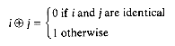
 j = 11010. (a b) = (a a) = b b) = a (b b) = a R1. For the leftmost node L1 = 0 and for the rightmost node R1 = 0. i n of a univariate polynomial, X, and to convert the polynomial into the circular linked list structure of section 4.4. Assume e1 > ei+1, 1 i < n, and that ci 0, 1 i n. Your algorithm should leave X pointing to the head node. Show that this operation can be performed in time O(n).
 will be put into the list for i and the node
  onto the list for j. Now process these lists outputting equivalence classes. With each class, output the relative position of each member of the class and check for conflicting equivalences .
Representation of matrix A of figure 4.11 using the scheme of exercise 22.
n. P is set to the starting address of the space allocated.ri M where M is the total amount of memory available, then all requests can be met. So, assume ri> M. storage allocated
----------------- get?
M
 log2n
log2n is allocated. As a result of this, all free blocks are also of size a power of 2. If the total memory size is 2m addressed from 0 to 2m - 1, then the possible sizes for free blocks are 2k, 0 k m. Free blocks of the same size will be maintained in the same available space list. Thus, this system will have m + 1 available space lists. Each list is a doubly linked circular list and has a head node AVAIL(i), 0 i m. Every free node has the following structure:
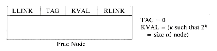 i m finding the smallest i for which AVAIL(i) is not empty. Remove one block from this list. Let P be the starting address of this block. If i > k, then the block is too big and is broken into two blocks of size 2i-1 beginning at P and P + 2i-1 respectively. The block beginning at P + 2i-1 is inserted into the corresponding available space list. If i - 1 > k, then the block is to be further split and so on. Finally, a block of size 2k beginning at P is allocated. A block in use has the form:
 2k where is the exclusive OR (XOR) operation defined in exercise 12. The is taken pair wise bit wise on the binary representation of y and 2k. 2k if the buddy is free. The new free block beginning at L = min {P,P 2k}and of size k + 1 is to be combined with its buddy L 2k+1 if free and so on. Write an algorithm to free a block beginning at P and having KVAL k combining buddies that are free.ni where ni is actual amount requested. Give an example approaching this ratio.
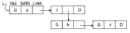
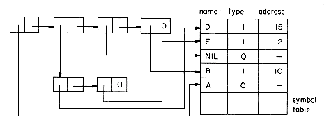
 'is returned if there are no more tokens.) i m. Show that this can be done in two phases, where in the first phase a left to right scan for free nodes and a right to left scan for nodes in use is carried out. During this phase, used nodes from the right end of memory are moved to free positions at the left end. The relocated address of such nodes is noted in one of the fields of the old address. At the end of this phase all nodes in use occupy a contiguous chunk of memory at the left end. In the second phase links to relocated nodes are updated. to fill up any unused space in a node. i j and xj < yj or if xi = yi for 1 i m and m < n. Write an algorithm which takes two strings X,Y and returns either -1, 0, +1 if X < Y, X = Y or X > Y respectively. j n and m > 1. Show using the definition of f that:
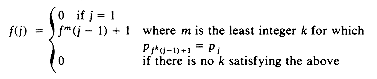
______________________
| | |
| Exponent | Link |
|_____________|________|
| Coefficient |
|______________________|
line 1: n m r n = # or rows
m = # or columns
r = # of nonzero terms
line 2
triples of (row, columns, value) on each line
line r + 1
