Formally, trees are collections of nodes. Trees derive both their appearance and their name from the lines, known as branches, that connect the nodes. Understanding how to represent trees, and how to perform certain operations on them, opens the door to an appreciation of many elegant algorithms and useful techniques in computer science.
Trees play a significant role in the organization of data for efficient information retrieval and are ideal candidates for fast searches, insertions, deletions, and sequential access. Efficiency and speed are possible because trees "spread out" the data they store, so that different paths in the tree lead quickly to the relevant data. They are also convenient for conceptualizing algorithms.
Many problems can be solved by imagining all the possible answers, represented as a tree. The algorithm or program is then viewed as a traversal through the tree. The general procedure for a traversal through a tree, which will be developed in this chapter, can then be adapted and used as the basis for the program. This often results in easily created and efficient programs. In such cases the tree itself serves as a conceptual aid and need not actually be "grown" or stored in memory. Nevertheless, it provides the framework for obtaining the algorithm.
The mathematics of trees has always been of interest and is discussed quite thoroughly by Knuth [1973a]. In this chapter we consider fundamentals and introduce special trees as they are needed in subsequent chapters.
As indicated in Figure 7.1, there are many ways to depict inclusion or hierarchical relationships. Each part of the figure conveys the same information about the relations between objects A to J. Figure 7.1(a) uses indentation reminiscent of program structure, or Pascal, COBOL, and C record structure, to convey inclusion. Figure 7.1(b) uses nested blocks or sets, while Figure 7.1(c) has nested parentheses. The last, Figure 7.1(d), uses lines that branch out like a tree turned upside down. This is how the data structure that is the topic of this chapter, the tree, is depicted.
If Figure 7.1(a) is being used to represent the structure of a C record, then the structure shows that record A includes three fields, B, C, and D, or that D includes two subfields, I and J. The tree of Figure 7.1(d) captures this inclusion information. To a C compiler, it is also important that field B comes before C and that C precedes D. When such ordering information is needed, we use ordered trees. To capture order, as well as inclusion information, Figure 7.1(d) must be an ordered tree.
Much of the terminology for the tree data structure is taken from botany and is therefore familiar and colorful. For instance, A of the tree in Figure 7.1(d) is at the root of the tree. The tree consists of three subtrees, whose roots contain B, C, and D. The entries in the tree, A to J, are each stored at a node of the tree, connected by lines called branches. The tree is ordered if each node has a specified first, second, or nth subtree. The order itself may be specified in many ways. In this example, the order is specified by taking the subtrees in alphabetical order, determined by their root entries. Rearranging the order of the subtrees in Figure 7.1(d) results in the same tree but not the same ordered tree, if we assume the ordering is specified for each node from left to right by the way the tree is pictured. A distinction will be made between ordered trees and trees throughout this text. Keep in mind that these terms refer to two distinct kinds of structures.
Besides these two kinds of trees, there are binary trees. A binary tree is either
n The null binary tree, or
n A root node and its left and right subtrees, which are themselves binary trees with no common nodes
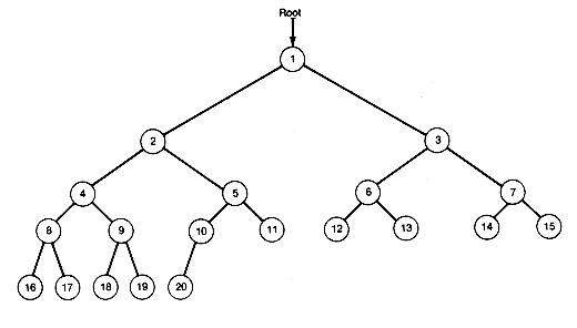
This recursive definition emphasizes the fact that binary trees with at least one node are composed of a root and two other binary trees, called the left and right subtrees, respectively. These subtrees, in turn, have the same structure. All binary trees consist of nodes, except for the null binary tree, which has no nodes. The null binary tree, just like the null list, cannot be "drawn." Both are used to make definitions more uniform and easier, and both represent the smallest data structure of their kind. There is exactly one binary tree with one node, its root. This tree has null left and right subtrees. The two binary trees with exactly two nodes are pictured as in Figure 7.2. One has a root and a nonnull left subtree, the other a root and a nonnull right subtree. Figure 7.3 pictures a larger binary tree.
The lines used to indicate a left and right subtree are called branches. Branches show the relationship between nodes and their subtrees. In Figure 7.3 the nodes are numbered 1 to 20 for easy reference. Node 5 has a predecessor (node 2), a left successor (node 10), and a right successor (node 11). Every node has at most two successors, and every node except the node labeled root has exactly one predecessor. Predecessors are also known as "parents," successors can be called "children," and nodes with the same parent are (what else?) "siblings." As far as is known, trees do not exhibit sibling rivalry.
Notice that, starting from any node in the tree, there is exactly one path from the node back to the root. This path is traveled by following the sequence of predecessors of the original node until the root is reached. For node 18, the sequence of predecessors is 9, 4, 2, and 1. There is always exactly one path from the root to any node.
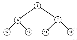
Follow the branch from node 1 to node 2 or 3 and you come to the left or right subtree of node 1. Its right subtree is shown in Figure 7.4. Similarly, each node has a left and a right subtree. Nodes with at least one successor are called internal nodes. Those with no successors are called terminal nodes (also known as "external" nodes or "leaf" nodes). The left and right subtrees of a terminal node are always null binary trees.
By definition, the root of a binary tree is at depth 1 . A node whose path to the root contains exactly d - 1 predecessor nodes has depth d. For example, node 10 in Figure 7.3 is at depth 4. This is the path length of the node. The longest path length is called the depth of the binary tree; it is 5 for the tree of Figure 7.3. For many applications it is the depth of a binary tree, like the depth of a list-structure, that determines the required storage and execution time.
Suppose your program must count the number of occurrences of each integer appearing in an input sequence of integers known to be between zero and 100. This is easy. Store the count for each integer of the allowed range in an array and increment the appropriate entry by 1 for each integer as it is input. The code would be array [i] + +, where i is the variable containing the integer just read. Note that the efficiency of this solution derives from the selection operation for an entry, which is supported by the array data structure.
What if the range of the integers was not known? Sufficient storage is not available for an array to store counts for all possible integers. What is required is a data structure that can be dynamically extended to accommodate each new integer and its count as the integer is encountered in the input. This data structure must be searched to see if the new integer already appears. If it does, its count is increased by 1 . Should the integer not appear, it must be inserted with its count set to 1. A special tree, a binary search tree introduced in Chapter 9, is convenient to use for this data structure. This tree allows the search for an integer to consider only nodes along a particular path. At worst, this path must be followed from the root to a terminal node. Thus the longest search time will be determined by the depth of the tree. The same data structure and the depth measure are important for the related problem, "Produce an index for a book." Now, instead of storing integer counts, the position of each occurrence of a word must be retained. Do you see the possibility of storing dictionaries of modest size in binary search trees?
Binary trees need not have such a compact look as that of Figure 7.3 but can appear sparse, as in Figure 7.5. A compact binary tree like Figure 7.3 is called a complete binary tree. To be more precise, a binary tree of depth d is a complete binary tree when it has terminal nodes only at the two greatest depths. d and d -1. Further, any nodes at the greatest depth occur to the left, and any nodes at depth less than d - 1 have two successors. In Figure 7.3, nodes 16 to 20 are the nodes at greatest depth; they occur to the left. The sparse tree has the same number of nodes but twice the depth.

Figure 7.1 Capturing Inclusion Relationships

(a) Left Subtree

(b) Right Subtree
Figure 7.2 Two Two-Node Binary Trees

Figure 7.3 A Binary Tree

Figure 7.4 The Right Subtree of the Root of Figure 7.3

Figure 7.5 A Sparse Binary Tree