


All data structures provide a way to organize data. Different structures serve different purposes. Complex lists, as shown by the information retrieval case study of Chapter 6, can result in considerable intertwining and sharing of lists and data. Everyone is familiar with the concept of a family tree. In fact, a nice exercise would be to print the family tree for an individual whose family history is stored in the data base of that case study. The family tree is actually embedded within the lists containing the family history. Trees may be viewed as a special case of lists in which no intertwining or sharing takes place. They are the basis for structures and operations used in all aspects of programming, from the structure of programs for compilers, to work in data processing, information retrieval, and artificial intelligence. Trees are ubiquitous; they seem to sprout everywhere--even in the field of computer science!
Formally, trees are collections of nodes. Trees derive both their appearance and their name from the lines, known as branches, that connect the nodes. Understanding how to represent trees, and how to perform certain operations on them, opens the door to an appreciation of many elegant algorithms and useful techniques in computer science.
Trees play a significant role in the organization of data for efficient information retrieval and are ideal candidates for fast searches, insertions, deletions, and sequential access. Efficiency and speed are possible because trees "spread out" the data they store, so that different paths in the tree lead quickly to the relevant data. They are also convenient for conceptualizing algorithms.
Many problems can be solved by imagining all the possible answers, represented as a tree. The algorithm or program is then viewed as a traversal through the tree. The general procedure for a traversal through a tree, which will be developed in this chapter, can then be adapted and used as the basis for the program. This often results in easily created and efficient programs. In such cases the tree itself serves as a conceptual aid and need not actually be "grown" or stored in memory. Nevertheless, it provides the framework for obtaining the algorithm.
The mathematics of trees has always been of interest and is discussed quite thoroughly by Knuth [1973a]. In this chapter we consider fundamentals and introduce special trees as they are needed in subsequent chapters.
As indicated in Figure 7.1, there are many ways to depict inclusion or hierarchical relationships. Each part of the figure conveys the same information about the relations between objects A to J. Figure 7.1(a) uses indentation reminiscent of program structure, or Pascal, COBOL, and C record structure, to convey inclusion. Figure 7.1(b) uses nested blocks or sets, while Figure 7.1(c) has nested parentheses. The last, Figure 7.1(d), uses lines that branch out like a tree turned upside down. This is how the data structure that is the topic of this chapter, the tree, is depicted.
If Figure 7.1(a) is being used to represent the structure of a C record, then the structure shows that record A includes three fields, B, C, and D, or that D includes two subfields, I and J. The tree of Figure 7.1(d) captures this inclusion information. To a C compiler, it is also important that field B comes before C and that C precedes D. When such ordering information is needed, we use ordered trees. To capture order, as well as inclusion information, Figure 7.1(d) must be an ordered tree.
Much of the terminology for the tree data structure is taken from botany and is therefore familiar and colorful. For instance, A of the tree in Figure 7.1(d) is at the root of the tree. The tree consists of three subtrees, whose roots contain B, C, and D. The entries in the tree, A to J, are each stored at a node of the tree, connected by lines called branches. The tree is ordered if each node has a specified first, second, or nth subtree. The order itself may be specified in many ways. In this example, the order is specified by taking the subtrees in alphabetical order, determined by their root entries. Rearranging the order of the subtrees in Figure 7.1(d) results in the same tree but not the same ordered tree, if we assume the ordering is specified for each node from left to right by the way the tree is pictured. A distinction will be made between ordered trees and trees throughout this text. Keep in mind that these terms refer to two distinct kinds of structures.
Besides these two kinds of trees, there are binary trees. A binary tree is either
The null binary tree, or
A root node and its left and right subtrees, which are themselves binary trees with no common nodes
This recursive definition emphasizes the fact that binary trees with at least one node are composed of a root and two other binary trees, called the left and right subtrees, respectively. These subtrees, in turn, have the same structure. All binary trees consist of nodes, except for the null binary tree, which has no nodes. The null binary tree, just like the null list, cannot be "drawn." Both are used to make definitions more uniform and easier, and both represent the smallest data structure of their kind. There is exactly one binary tree with one node, its root. This tree has null left and right subtrees. The two binary trees with exactly two nodes are pictured as in Figure 7.2. One has a root and a nonnull left subtree, the other a root and a nonnull right subtree. Figure 7.3 pictures a larger binary tree.
The lines used to indicate a left and right subtree are called branches. Branches show the relationship between nodes and their subtrees. In Figure 7.3 the nodes are numbered 1 to 20 for easy reference. Node 5 has a predecessor (node 2), a left successor (node 10), and a right successor (node 11). Every node has at most two successors, and every node except the node labeled root has exactly one predecessor. Predecessors are also known as "parents," successors can be called "children," and nodes with the same parent are (what else?) "siblings." As far as is known, trees do not exhibit sibling rivalry.
Notice that, starting from any node in the tree, there is exactly one path from the node back to the root. This path is traveled by following the sequence of predecessors of the original node until the root is reached. For node 18, the sequence of predecessors is 9, 4, 2, and 1. There is always exactly one path from the root to any node.
Follow the branch from node 1 to node 2 or 3 and you come to the left or right subtree of node 1. Its right subtree is shown in Figure 7.4. Similarly, each node has a left and a right subtree. Nodes with at least one successor are called internal nodes. Those with no successors are called terminal nodes (also known as "external" nodes or "leaf" nodes). The left and right subtrees of a terminal node are always null binary trees.
By definition, the root of a binary tree is at depth 1 . A node whose path to the root contains exactly d - 1 predecessor nodes has depth d. For example, node 10 in Figure 7.3 is at depth 4. This is the path length of the node. The longest path length is called the depth of the binary tree; it is 5 for the tree of Figure 7.3. For many applications it is the depth of a binary tree, like the depth of a list-structure, that determines the required storage and execution time.
Suppose your program must count the number of occurrences of each integer appearing in an input sequence of integers known to be between zero and 100. This is easy. Store the count for each integer of the allowed range in an array and increment the appropriate entry by 1 for each integer as it is input. The code would be array [i] + +, where i is the variable containing the integer just read. Note that the efficiency of this solution derives from the selection operation for an entry, which is supported by the array data structure.
What if the range of the integers was not known? Sufficient storage is not available for an array to store counts for all possible integers. What is required is a data structure that can be dynamically extended to accommodate each new integer and its count as the integer is encountered in the input. This data structure must be searched to see if the new integer already appears. If it does, its count is increased by 1 . Should the integer not appear, it must be inserted with its count set to 1. A special tree, a binary search tree introduced in Chapter 9, is convenient to use for this data structure. This tree allows the search for an integer to consider only nodes along a particular path. At worst, this path must be followed from the root to a terminal node. Thus the longest search time will be determined by the depth of the tree. The same data structure and the depth measure are important for the related problem, "Produce an index for a book." Now, instead of storing integer counts, the position of each occurrence of a word must be retained. Do you see the possibility of storing dictionaries of modest size in binary search trees?
Binary trees need not have such a compact look as that of Figure 7.3 but can appear sparse, as in Figure 7.5. A compact binary tree like Figure 7.3 is called a complete binary tree. To be more precise, a binary tree of depth d is a complete binary tree when it has terminal nodes only at the two greatest depths. d and d -1. Further, any nodes at the greatest depth occur to the left, and any nodes at depth less than d - 1 have two successors. In Figure 7.3, nodes 16 to 20 are the nodes at greatest depth; they occur to the left. The sparse tree has the same number of nodes but twice the depth.
*This section can be omitted on first reading.
Let us take a moment here to derive two important relations between the depth, d and the number of nodes, n, in a binary tree. First note that in any binary tree there is at most one node at depth 1, at most two nodes at depth 2, and, in general, at most 2k-1 nodes at depth k, since a node can give rise to at most two nodes at the next depth. The total number of nodes, n, is then at most 1 + 21 + 22 + . . . + 2d-1. This sum is 2d - 1. So
The minimum possible depth, dmin, for a binary tree with n nodes will be given by
where
The nodes of binary trees may be used to store information. For example, the nametable of Section 6.5 could be implemented by storing each of its records at a node of a binary tree. Just as lists are referred to by name, the tree can be named, say nametable. Obviously, nametable must have records inserted into it, deleted from it, and searched for in it. Insertion, deletion, search, and traversal are the basic tree operations.
Balanced trees and binary search trees (Chapter 9) and heaps (Chapter 8) are all binary trees with special properties that make them useful for storage of information. The properties that make them useful favor efficient searching, inserting, and deleting. Each of these types of binary tree requires its own algorithms for these operations, in order to take advantage of or to preserve their characteristics. For now, to get the flavor of these operations, consider some simple examples.
Assume that each node of a binary tree is represented by a record containing an information field, a left pointer field, and a right pointer field. The notation node.p stands for the record or node pointed to by the variable p.
To accomplish an insertion, storage must first be allocated for a new record. Next, its fields must be set correctly; this includes entering data into the record and setting its pointers to the succeeding left and right nodes, or to null if it is a leaf. Finally the proper pointer adjustments must be made in the tree to the predecessor of the new entry. Consider Figure 7.6, which shows a binary tree t before and after the insertion of a new entry C, which replaces predecessor O's null right subtree. The information for the new record is assumed to reside in value, so C is stored in value. Thus the new record must have its information field set to value and its left and right pointer fields set to null. The predecessor's right pointer field must be set to point to the new record. This is accomplished by the following.
Setinfo copies the contents of the storage pointed to by its second parameter into the info field of the record pointed to by its first parameter. Note that it is defined somewhat differently from the setinfo used in previous chapters. Setleft and setright copy the contents of their second parameter into the proper field of the record pointed to by their first parameter. Notice that setleft is used to set the left pointer of the new record; similarly for setright. However, setright is also used to change the right pointer of the predecessor record so that it points to the new record, which is now its right node. Thus setleft and setright can be used to set pointers for any node in the tree. Together with setinfo and avail, these functions reflect the binary tree's implementation details. The code for the insertion itself is independent of the implementation.
If a new record is to replace a nonnull subtree (say, if C were to replace U in t), then the new record's left and right pointer fields would have to be adjusted accordingly. The left and right pointers from U would have to be copied into the new record's (C's) pointer fields. Furthermore, the storage for the replaced record U might be reclaimable. If so, care is required to save the pointer to it in its predecessor's left or right field so that its storage can be reclaimed. In this example, after saving the pointer to U, the right pointer of U's predecessor, L, would be replaced by a pointer to C, its new right node. Then U's storage can be reclaimed. The code below does this correctly, assuming predecessor points to a record whose nonnull right subtree is to be replaced.
Right returns a copy of the right pointer field value of the record pointed to by its parameter. This code is for illustrative purposes. If the record is really reclaimable, it would be more efficient simply to replace its info field by the new info value. The statement setinfo(q,&value) would suffice. However, if the replaced record were needed for another purpose, say for insertion in another binary tree, then this would not work.
The deletion of a terminal node pointed to by p, whose predecessor is pointed to by predecessor, may be accomplished by the following.
Left is analogous to right. The decision is required in order to know whether it is predecessor's left or right successor that is to be deleted. Again, if the deleted node's storage may be reclaimed, care must be taken not to lose the pointer to it. Deletion of an internal node must take into account what is to be done with the node's subtrees.
The wary reader may have qualms about the code developed for insertion and deletion. Remember--special cases must always be checked. When insertion or deletion occurs at the root node, indicated by a null value in predecessor, it is the name of the tree whose pointer must be adjusted. The illustrative code fails in this case. You should modify the program segments so that they also account for this special case.
We have seen examples whose solution includes a traversal through a collection of records in an array or a list. A traversal through a collection of records stored in a binary tree is also the basis for the solution to many problems. We will consider three distinct ways to traverse a binary tree: (1) preorder, (2) inorder, and (3)postorder.
Pre-, in-, and postorder traversals are often referred to mnemonically as root-left-right, left-root-right, and left-right-root traversals. The prefixes pre, in, and post refer to whether the root is accessed prior to, in between, or after the corresponding traversals of the left and right subtrees. In all cases, the left subtree is traversed before the right subtree. When nodes are listed in the order in which they are processed, all nodes in the left subtree appear before all nodes in the right subtree, no matter which traversal is used. However, the type of traversal determines where the root appears. Since we defined binary trees recursively, it is convenient to give recursive definitions for these traversals.
To preorder traverse a binary tree:
if the binary tree is not the null binary tree, then
1. access and process its root
2. traverse its left subtree in preorder
3. traverse its right subtree in preorder
To inorder traverse a binary tree:
if the binary tree is not the null binary tree, then
1. traverse its left subtree in inorder
2. access and process its root
3. traverse its right subtree in inorder
To postorder traverse a binary tree:
if the binary tree is not the null binary tree, then
1. traverse its left subtree in postorder
2. traverse its right subtree in postorder
3. access and process its root
Let's apply these definitions to Figure 7.6(b).
To do a preorder traversal of t, since it is not null, requires that its root, L, be accessed and processed first. Next, the left subtree of t must be preorder traversed. Applying the definition to it, its root, O, is accessed and processed. Since O's left subtree is null, its right subtree is traversed next in preorder. This results in C being accessed and processed, terminating the preorder traversal of O's right subtree and also of t's left subtree. Completing t's traversal requires a preorder traversal of its right subtree, resulting in U, S, and T being accessed and processed in turn.
An inorder traversal of t requires its left subtree to be inorder traversed first. Applying the definition to this left subtree requires its null left subtree to be inorder traversed (note how easy that is), its root O to be accessed and processed next, and then its right subtree to be inorder traversed, which results in C being accessed and processed. This terminates the inorder traversal of t's left subtree. T's root, L, must then be accessed and processed, followed by an inorder traversal of t's right subtree. This causes S, U, and T to be accessed and processed in turn, completing the inorder traversal of t.
Try applying the postorder traversal definition to t yourself. The sequences below represent the order in which the records stored at the nodes of t are accessed and processed for each of the traversals.
Notice that the terminal nodes C, S, and T are dealt with in the same order for all three traversals. This is not just a coincidence but will always happen.
The trees of Figure 7.7 represent a table of contents, an arithmetic expression, and a program that invokes functions that, in turn, invoke other functions. Traversing these trees, respectively, in pre-, in-, and postorder results in the order of access to nodes shown in Figure 7.7(d-f). Each is a natural application of one of the three traversals: a listing of the table of contents, an arithmetic expression in the usual notation, and a listing of the order in which the functions are needed to test another function (for example, P1 and P2 are needed to test P3).
Not all data structures need to be traversed. For example, stacks, queues, heaps, and the hash tables to be introduced in Chapter 9 are not normally traversed. Just as applications of arrays and, even more so, lists often reduce to traversals, applications of binary trees often do as well. Therefore procedures for their traversal merit study.
Writing a recursive function to traverse a binary tree based on the recursive definition for preorder traversal is straightforward. The same is true for an inorder and postorder traversal.
Recursive Version
To convince yourself it works, simulate it on the tree of Figure 7.6(b).
We will now develop an iterative procedure for contrast with the recursive one. It will also be useful if the programming language you are using is not recursive. Recall that the application of the definition of preorder traversal to Figure 7.6(b) required keeping track of the left subtree about to be traversed and remembering at which node to resume when that left subtree traversal terminated. For example, in Figure 7.6(b), after node L is processed, its left subtree must be preorder traversed. We must remember, after that traversal is complete, to resume the traversal by traversing L's right subtree. Put another way, it was necessary to suspend the current traversal, incurring its completion as a postponed obligation, and begin a traversal of the proper left subtree. These postponed obligations must be recalled and resumed in reverse order to the order in which they were incurred. That is, in a last-in first-out fashion. Obviously, the ubiquitous stack is called for. It seems to pop up everywhere.
To accomplish this let p point to the root of the subtree about to be traversed. After the processing of node.p, a pointer to its right subtree can be pushed onto the stack before traversal of its left subtree. At the time that node.p's right subtree is to be processed (when its left subtree traversal terminates), the stack will contain pointers to all right subtrees whose traversals have been postponed (right subtrees of nodes already accessed), but the top stack entry will point to node.p's right subtree. Thus popping the stack and setting p to the popped value correctly updates p to point to the correct next record to be accessed.
Nonrecursive Version Saving Right Pointers on a Stack
The while loop condition is true whenever the traversal is not yet completed. A nonnull p means that a record is pointed to by p and is the next one to be accessed and processed. A null p value means no record is pointed to by p, and some left subtree traversal must have just been completed. If, at that point, the stack is not empty, then more needs to be done; but if it is empty, then no right subtrees remain to be traversed, and the traversal is done. Again, to convince yourself the program works, simulate it on the tree of Figure 7.6(b).
The recursive procedure reflects the structure of binary trees and emphasizes that they are made up of a root with binary trees as subtrees. It sees the special cases, such as a null tree, and the substructures of the recursive definition, such as left and right subtrees. In order to develop the nonrecursive version, it is necessary to think of the binary tree as a collection of individual records. Writing the function then involves providing for the correct next record to be accessed and processed within the while loop. This is a general strategy for attempting to find nonrecursive solutions. The nonrecursive version requires that the structure be viewed as a collection of its individual parts, with each part treated appropriately and in the correct order. This explains why recursive versions are clearer.
An alternative nonrecursive function is based on saving on a stack the path from the root to the predecessor of the node currently being processed. It is useful if the processing of a node requires accessing its predecessor node. This alternative approach guarantees that at the time the node is processed its predecessor is at the top of the stack. However, this algorithm requires some searching to find the proper right subtree to traverse next when a subtree traversal has terminated. Such a termination is indicated by p being null. Figure 7.8 shows a situation when such a termination has occurred. P is null, having been set to the null right pointer value of node 10 after node 10's left subtree has been traversed. Looking back along the path from node 10 to the root, we find the path nodes 8, 6, 5, 1. It is not difficult to see that node 5's right subtree is where the traversal must resume. Precisely this path back toward the root must be followed until a node on this return path (node 6) is the left successor of its predecessor. P must then be set to the right subtree of that node (node 12) and the traversal resumed. If no node which is the left successor of its predecessor is found on the return path, the entire tree has been traversed.
The following function is a nonrecursive preorder traversal that saves the path to the root on a stack. Item returns a copy of the pointer at the top of the stack without disturbing the stack.
Nonrecursive Version Saving the Path to the Root on a Stack
Notice that the first two versions of the preorder traversal do not retain information about the depth of a node or about a node's predecessor, although they could be modified to do so. The third version retains this information, since the depth of the current node is equal to the number of stack entries plus one, and the top stack entry always points to the current node's predecessor. When this information is needed, the last version provides it directly, especially if a basic stack operation that returns the size of the stack is available.
Each of the three traversal functions can be modified to be a partial traversal when required, by including a variable done to signal termination, just as was done for the list traversals. This would be the case, for example, if you were traversing only to find a desired record. Similar function can be written for the inorder and postorder traversals.
In this section a number of examples are presented to show how the traverse functions developed thus far can be applied to develop solutions to programming problems.
Example 7.1
Print the number of terminal nodes in a binary tree tree.
The nonrecursive preorder traversal that saves right subtree pointers on a stack will be used to perform this task. The other versions could have been adapted as readily. The approach taken is to leave the traverse function as it is and write process to turn preorder into a solution to the problem.
To accomplish this, process must test each node it deals with to see if it is a terminal node. If so a counter, tncount, should be increased by 1. Making tncount a static variable in process allows its values to be preserved between calls to process. The first time process is called during the traversal it must initialize tncount to zero, and the last time it is called, in addition to updating tncount, process must print its final value.
If p points to the current record to be processed, then when p points to the root of the traversed tree tree, process has been called for the first time, so it must set tncount to zero. But how can process recognize when p points to the last node so that tncount can be printed? To do this, process must have access to the stack s. When s contains no nonnull pointers and node.p is a terminal node, then node.p is the last node. Assume that a function last returns true if s contains no nonnull pointers and false otherwise. Consequently s must be a parameter of, or global to, process. Finally, we must assume that only nonnull binary trees are to be considered since process is invoked by preorder only when tree is not null. Process may now be defined as follows.
It would certainly be more efficient to make null global so that setnull would not be invoked for each node. Similarly, setting tncount to zero in preorder could remove the need for the (p == *ptree) test for each node. In fact, it would be easier to take a second approach to finding a solution. Namely, modify preorder so that it sets tncount to zero initially, and after its while loop is exited, simply print tncount. This second solution is considerably more efficient, because the test performed by last is not needed. The second approach is more efficient, but it involves changing a traversal, which may be already compiled. Which approach to use depends on what alternatives are available and just how important the extra efficiency is.
Example 7.2
The second example concerns the problem of inserting a new node in the binary tree tree in place of the first terminal node encountered in a preorder traversal of tree. The information field value of the new node is to be copied from that of the record value.
In this case process will be written to make a solution out of the nonrecursive version of preorder that stores the path from the root to the node being processed. This is convenient, since the predecessor of the node to be processed is required by process when the insertion is made, and it will be the top stack entry at that time.
When process is called, it tests whether the node is a terminal node. Since it will cause the traversal to be terminated after the replacement, this must be the first terminal node. Storage is then obtained for the new record and its fields filled in properly. Since it will be a terminal node, its pointer fields are set to null. To insert the new record, the predecessor of the terminal node must have one of its pointer fields set to point to the new record. The correct one is determined by whether the replaced record was its left or right successor. The special case of the insertion occurring at the root requires only that tree be set to point to the new record. Finally, setting the stack to empty ensures that the traversal will be aborted.
Value is passed by preorder to process. Item simply returns a copy of the top stack entry.
Example 7.3
The final example involves writing a function depth to return the depth of a binary tree as its value.
The nonrecursive version of preorder that saves the path to the root on the stack can be turned into such a function. When a node is being processed, its depth is one more than the number of stack entries at that moment. To determine the depth, initialize a variable d to 1 and size to zero before the while loop, increase size by 1 after push, and decrease it by 1 after pop. Give process access to d and size. Process must simply compare size+1 to d, and when greater, set d to size+1. After termination of the traversal, depth must return d.
Another solution for depth can be obtained by recursion. This requires a way to express the depth recursively. The depth of a binary tree t is
Zero if t is null, else
One more than the maximum of the depths of t's left and right subtrees
Now the function can be written directly as follows:
where max returns the maximum of its parameters as its value.
This section introduces three ways to implement a binary tree.
1. Using an array of records with just an information field
2. Using records with an information field and left and right pointer fields linked together via their pointer fields
3. Using a list-structure
Chapter 8 contains an application of the first implementation. A program using the second implementation, with the records stored in dynamic memory, is included. The program specifies the details of this important representation and illustrates how to create and process binary trees and how to test functions developed in the earlier examples.
The sequential representation uses an array to store information corresponding to each node of a tree. Consider the binary tree shown in Figure 7.9. Its depth is 5 and it has fourteen nodes. The nodes are numbered in a special way. This numbering may be obtained by preorder traversing the tree and, as each node is accessed, assigning it a node number. The root is assigned 1, each left successor of a node is assigned twice the number of its predecessor, and each right successor is assigned one more than twice the number of its predecessor. With nodes numbered in this way, the predecessor of node i is numbered i/2 (integer divide), its left successor is numbered 2*i, and its right successor 2*i+1.
The sequential representation of a binary tree is obtained by storing the record corresponding to node i of the tree as the ith record in an array of records, as shown in Figure 7.9. A node not in the tree can be recognized by a special value in its corresponding array position (such as node 8, which has - as its value) or by a node number (like 24) that exceeds the highest node number in the tree (20 in this example). Given a pointer p to a node in the array, it is easy to determine the position of its predecessor (p/2), its left successor (2*p), and its right successor (2*p+1).
A binary tree with n nodes will require an array length between n and 2n - 1. The smallest length (n) is sufficient when the binary tree is complete, and the greatest length (2n - 1) corresponds to the case of an extremely skewed binary tree whose nodes have only right successors. No space in the array is unused for a complete binary tree, and the array length is proportional to the number of nodes in the tree. However, a sparse tree can waste a great deal of array space. The worst case requires 2n - 1 positions but uses only n. Thus the sequential representation is convenient for dealing with complete static binary trees. Such trees arise, for example, when you must put student records in alphabetical order by student name. How to do such ordering is considered in the next chapter (Section 8.4). For cases when the tree may change size or shape drastically, the sequential representation is not appropriate. An example of this situation is found in the integer or word counting problem of Section 7.1.
A binary tree data structure can also be implemented by representing each node of the tree as a record with three fields:
1. A left pointer field,
2. An information field
3. A right pointer field
(called here the leftptr, info, and rightptr fields). This is the most common representation. The left and right pointer fields link records of the tree, just as the link and sublist fields of lists link their records. In effect, the pointer fields specify a node's left and right subtrees, just as the sublist field of a list specifies its sublist. The leftptr and rightptr fields of a node point to the record that represents, respectively, the root of the node's left and right subtree. The info field contains the information stored at the node. A variable referred to as the name of the tree points to the record representing the root of the tree, and a null pointer in the name denotes the null tree.
We can store each record of a binary tree using an array of records as shown in Figure 7.10, just as was done for the records of lists. The binary tree fred, for example, has its root stored in position 5 of the array, while the root of t is in position 2. the left successor of fred's root is stored in position 8, and its right successor in position 0. A minus one is used as the null pointer.
The definitions for the records and the array declaration are as follows.
Instead of using an array and array indices, we may store the records of the tree in dynamic memory and use pointers. The record declarations then become
Such linked representations require storage proportional to the number of nodes of the binary tree represented, no matter what the shape of the binary tree. Contrast this with the sequential representation of binary trees. If a linked representation uses three elements per record, whereas a sequential representation uses one element per record, then for complete binary trees three times as much storage is used in a linked representation as in a sequential one. If the binary tree is not complete, then the sequential representation may require storage proportional to 2d - 1, where d is the depth of the binary tree. This could result in significant amounts of wasted space; there may not even be enough storage. Consequently, the sequential representation is more practical only when dealing with complete or nonsparse binary trees.
Using the linked representation, it is obviously possible to insert or delete records, once we know where to do so, by making changes in only a few pointer fields.
The following program illustrates the binary tree implementation with records stored in dynamic memory. It is a program that could be used to test all the functions of Section 7.3 (although they have been renamed). The names are self-explanatory. The input consists of
An integer to indicate whether the binary tree being created is null,
A sequence of data for each record
A value for the info field of a new node
The sequence is assumed to be in the order in which the records are accessed in a preorder traversal of the binary tree being input. For example, if the input corresponded to the right subtree of Figure 7.9 and the new value replacing the first terminal node were 50, then the input would be as follows. (Program output and prompts are not shown.)
Typical Input
The Program
Another way to represent a binary tree is indicated in Figure 7.11. Each node's record is made complex. A complex record's sublist points to the representation of the node's left subtree. The result is that btree is implemented as the list structure lstree. Abstractly, binary trees are a special case of list-structures, but there are list-structures that do not correspond to binary trees. However, in computer science the term tree usually implies zero or restricted sharing of storage, whereas the term list-structure or list implies the possibility of more general sharing of storage.
So far we have considered only binary trees, but trees may have nodes with more than two successors. This is the case in the tree of Figure 7.1, where the nodes have up to three successors. It would be natural to assume that binary trees are a special case of trees, but the tree literature does not treat them this way. The formal definition of a tree, as opposed to a binary tree, is as follows: A tree is a root node with subtrees t1, t2, . . . , tn that are themselves trees and have no nodes in common.
Formally there are no null trees (although there are null binary trees), so each tree has at least one node, its root. It is convenient nonetheless to refer to null trees, so the terminology applied to binary trees also applies to trees. The important distinction is that no order is imposed on the subtrees of a tree, whereas for binary trees there is a distinct left and right subtree. Consequently, when trees are depicted, it makes no difference in what order subtrees are drawn; any order represents the same tree. When order among the subtrees is to be imposed, they are called ordered trees. For example the structures in Figure 7.12, when viewed as binary trees, represent two distinct binary trees, since their left and right subtrees differ, but they represent the same tree when viewed as trees.
When a constraint is imposed limiting the number of successors of any node to at most k, the tree is called a k-ary tree. Such trees may be implemented by generalizing the sequential representation for binary trees. The nodes are numbered as before, except the jth successor of the node numbered i is now assigned node number k X (i - 1) + (j + 1). Thus, when k = 5, the fourth successor (j = 4) of the node numbered i (i = 3) is assigned the number 5*(3 - 1) + (4 + 1) = 15. A 5-ary tree with nodes numbered in this way is
This implementation will not be pursued further but is similar in character to the sequential implementation for binary trees. This means that formulas can be derived to compute the array position of a node's predecessor and successors, which are important requirements for tree processing. Also, this representation is convenient for essentially static, healthy-looking (nonparse) trees.
Another representation is based on a natural generalization of the linked representation for binary trees. Simply expand each record so that it has as many pointer fields as it has subtrees. However, this leads to variable-length records, which are usually not desirable. The variable-length records occur because nodes need not all have the same number of successors. Further, it may not even be possible to predict in advance what the greatest number of successors will be.When it is known that the tree will be a k-ary tree, then all records could be made the same length, large enough to accommodate k subtree pointers. This gives a fixed record size but can result in considerable wasted storage for unused pointer fields within records. This is particularly true for sparse trees.
Surprisingly, there is a way to represent a tree as a binary tree, which then allows all records to be of fixed length. This is an important result. Since any tree can be represented by a binary tree, studying only binary trees is really no restriction at all.
Example 7.4
Let us now look at how to represent a specific tree as a binary tree. Consider the tree of Figure 7.13(a). How can this tree be represented as a binary tree?
The binary tree is obtained as follows: First, create a root A of the binary tree to correspond to the root A of the tree. Next, pick any successor of A in the tree--say, B--and create a node B in the binary tree as A's left successor. Then take the remaining siblings of B, which are C and D in this case, and let C be B's right successor and D be C's right successor, in the binary tree. So far this yields the binary tree shown in Figure 7.13(b). If we view this procedure as the processing of node A of the tree, then the binary tree is completed by repeating this procedure for every other node of the tree. For example, after node B is processed (that is, its successors have been added to the binary tree), the result is Figure 7.13(c). The final binary tree created using this procedure appears in Figure 7.13(d).
Applying this procedure, given any tree, a corresponding binary tree can be constructed. The specific binary tree generated will depend on the order in which successors are taken in the tree. For instance, had C been selected initially as the first successor of A, then the resultant binary tree would be different. If the ordering of each node's successors is specified and they are taken in the specified order, then the construction creates a unique binary tree for each tree. In any case, a tree with n nodes will correspond to a binary tree with n nodes. It is not difficult to find an algorithm that, given a binary tree with no right subtree, can reverse the construction and generate the tree it represents. This means that when the tree is ordered, there is a unique binary tree that can be constructed to represent it. Conversely, given a binary tree with no right subtree, there is a unique tree that it represents, which can also be constructed. Hence there are exactly as many trees with n nodes as there are binary trees with n nodes and no right subtrees.
If we define an ordered forest as an ordered collection of ordered trees, then each tree has its unique binary tree representation. Can you see how to append these binary trees to the binary tree representing the first ordered tree of the ordered forest to obtain a binary tree representing the forest? (Hint: Use the fact that the binary trees have no right subtrees.) For those of you who wish to count trees, pursuing this should lead to the conclusion that there are exactly as many ordered forests as there are binary trees.
In this section algorithms are developed for traversing trees and are applied to two examples. The second example should be studied carefully, because it illustrates an important modified traversal of trees that has many applications. Assuming the trees are ordered, it makes sense to refer to a tree's first subtree, second subtree, and so on. If an order is not given, the programmer can impose one.
When trees are used to store data at their nodes, then tree traversals give a means to access all the data. However, a tree might be used to represent a maze or all routes from Philadelphia to San Francisco. Traversal of the tree then provides the means to find exits from the maze or the shortest route across the country. The maze and the routes must not intersect. When they do, a more general data structure, a graph, is needed for their representation. Unlike trees, a graph allows more than one path between its nodes. * Should a tree contain family relationships by storing an individual's record at a node, a traversal allows the parent (predecessor) or the children (successors) of an individual to be found.
* It is not difficult to generalize tree traversal algorithms to obtain graph traversal algorithms.
The preorder and postorder traversals of binary trees generalize quite naturally to ordered trees.
To preorder traverse an ordered tree:
1. Access and process its root, then
2. Preorder traverse its subtrees in order.
To postorder traverse an ordered tree:
1. Postorder traverse its subtrees in order, then
2. Access and process its root.
There is no natural inorder traversal of trees. Preorder and postorder traversals of a tree correspond, respectively, to preorder and inorder traversals of its corresponding binary tree. The preorder and postorder access sequences for the tree of Figure 7.13(a) are ABEFGCHDIKLMJ and EFGBHCKLMIJDA. You should confirm that a preorder and an inorder traversal of the binary tree of Figure 7.13 result in these respective access sequences. A preorder traversal is also called a depth-first traversal.
It should now be clear that confining attention to binary trees, their representation, and operations on them is not actually a restriction. That is, since trees can be represented as binary trees, any operations can be performed on them by performing equivalent operations on their binary tree representations. In this sense no generality is lost in dealing with binary trees.
Example 7.5
Let the task for this example be the development of an algorithm to generate the binary tree corresponding to a general tree.
In order to do this we must be able to traverse a general tree. As it is traversed, we can generate the binary tree by properly processing each node as it is accessed. A nonrecursive algorithm to preorder traverse a tree t follows.
Nonrecursive Tree Preorder Traversal
1. Set p to t
2. Setstack_t(ts)
3. While p is not null or not empty_t(ts),
if p is not null, then
process(t,p)
For each successor pointer ps of node.p,
except next(p),
push_t(ps,ts)
Update p to next(p)
else
pop_t(ts,p)
This algorithm is a generalization of the nonrecursive preorder traversal of a binary tree that saves right pointers. In the binary tree case, the next subtree is the left subtree, and only one successor of the node just processed must be saved--the right successor. The difference is that now all the subtree pointers of the node just processed, except for the next one, must be saved.
Now that we have a general tree traversal, it will be adapted to our task. Let bt point to the binary tree to be generated by the algorithm. Recall the list-structure representation of a binary tree. Think of the leftpointer field of each node of bt as pointing to a sublist. This sublist contains all the successors of the corresponding node in t. Thus, in Figure 7.13(d), node A of the binary tree representation has a leftpointer field pointing to the sublist consisting of nodes B, C, and D. These are the successors of A in the general tree, Figure 7.13(a). Similarly, D has a leftpointer field pointing to the sublist consisting of I and J, the successors of D in the general tree.
Consequently, to produce bt, when a node of t is processed we must
Create a sublist consisting of all its successors
Set the leftpointer field of the corresponding node in bt to point to this sublist
Copy the info field of the node in t into the info field of the corresponding node in bt
The rightpointer fields of these nodes in bt serve as the link fields of the sublist.
Recall that, as we preorder traverse a general tree t, we are preorder traversing its corresponding binary tree, bt. That is, the order in which the nodes of t are accessed is exactly the same as the order in which the corresponding nodes of bt are accessed. Thus we can achieve a solution by preorder traversing both t and bt at the same time, and processing the corresponding nodes as described above. For example, if this were carried out on the general and final binary tree of Figure 7.13, and nodes A, B, E, F, G, and C had been processed, we would have generated the binary tree shown as Figure 7.14(b).
Suppose p points to the node currently being processed in t. Let pb point to the corresponding node in bt. In the example, p would now point to D of t and pb to D of bt.
After processing the node to which p points, we can update p to point to one of its successors, next(p), and stack on ts all pointers to the remaining successors. These pointers represent the latest postponed obligations for the preorder traversal of t. Next (p) is a function returning a pointer to the successor of p that is not stacked, or a null pointer if there are no successors. At the same time, to keep track of the postponed obligations for bt's preorder traversal, we will keep a parallel stack, bts. Only nonnull pointers will be pushed onto bts. When the top pointer in stack ts is popped, the top pointer in bts will also be popped. These pointers will then point to corresponding nodes--one in t, the other in bt. Storage can be created for the nodes of bt as the traversal proceeds by using avail to return a pointer to the available storage for a node, since a pointer variable implementation is used for the binary tree.
One last detail remains. In order to do the processing required on node.p and node.pb, process will be invoked. As already noted, process must create a sublist consisting of new nodes corresponding to the successors of node.p in t, set leftptr.pb to point to that sublist, and copy info.p into info.pb. We assume that a procedure create, given p, creates the required sublist, and returns with first pointing to the first node of that sublist. The preorder traversal algorithm to create the binary tree corresponding to a general tree is as follows:
Nonrecursive Algorithm to Generate a Binary Tree Corresponding to a General Tree
1. Set p to t
If p is null
Set bt to null
else
bt = avail()
Set pb to bt
2. Setstack_t(ts)
Setstack_bt(bts)
3. While p is not null or not empty_t(ts),
if p is not null, then
process(t,bt,p,pb).
For each successor pointer ps of node.p, except next(p),
push_t(ps,ts)
If right(pb) is not null
push_bt(right(pb),bts)
p = next(p)
pb = left(pb)
else
pop_t(ts,p)
pop_bt(bts,pb).
The process algorithm to be used in the preorder traversal is:
Create(p,first)
Set leftptr.pb to first
Set info.pb to info.p
Notice that the traversal of the binary tree bt is embedded in the traversal of the general tree t. Also, suffixes have been used to distinguish the stack storing pointers to nodes of the general tree from the stack storing pointers to nodes of the binary tree. Finally, since the tree t is not ordered, the function next is free to pick any successor. The order in which the rest of the successors are placed on the stack is arbitrary but must determine the order in which create places them on the sublist. You should simulate this algorithm on the tree of Figure 7.13(a) to see how it works.
The correspondence between an ordered tree and its binary tree can now be defined more formally. In this case the binary tree corresponding to a tree is unique. An ordered tree t may be represented by a binary tree bt as follows:
Each node of t corresponds to a node of bt,
If node n of t corresponds to node nb of bt, then the leftmost successor of n in t corresponds to the left successor of nb in bt;
All other siblings of n in t form a right chain from the node in bt corresponding to the leftmost successor of n in t.
We may now give a recursive definition specifying an algorithm for generating the binary tree bt representing the general ordered tree t.
To generate a binary tree corresponding to an ordered tree:
If t is null
Set bt to null
else
Create the root node of bt corresponding to the root of t.
If t has a subtree, then generate the binary tree bt.left corresponding to the leftmost subtree of t,t.leftmost, and make the generated binary tree the left subtree of bt.
For every other subtree of t, in order, generate the binary tree corresponding to the subtree, and insert it at the end of the right chain of bt.left.
For illustration this algorithm is applied to the ordered tree in t in Figure 7.15(a).
First create the root of BT corresponding to the root of t shown in Figure 7.15(b). To carry out statement 2, note that t has three subtrees with B at the root of its leftmost subtree. We must thus generate bt.left to orrespond to Figure 7.15(c). To do this, apply the definition to this tree and obtain Figure 7.15(d) as its corresponding binary tree. Completing the first part of statement 2 for t yields the binary tree shown in Figure 7.15(e).
To complete the second part of statement 2, generate the binary tree for the next subtree of t, with C at its root, and then insert it at the end of the right chain of B to obtain Figure 7.15(f). Finally, do the same for the last subtree of A, with D at its root, and complete the application to t, to obtain the result shown in Figure 7.15(g).
This is another example for which we found a recursive solution. Compare the clarity and conciseness of the recursive solution with that of the nonrecursive solution.
In the last section a tree traversal was developed and used to generate a binary tree. Here and in the following two sections we will develop a modified tree traversal that employs backtracking. Backtracking is a useful technique in solving many problems. First we apply it to the n-queens problem.
Chess is played on a square board with eight rows and eight columns, just like a checkerboard. We can think of the board as a two-dimensional array, board (Figure 7.16).
A queen located in the jth row and kth column may move to a new position in one of the following ways:
To the right, or left, along its row
Up, or down, in its column
Up, or down, along its d1 diagonal
Up, or down, along its d2 diagonal
The n-queens problem is to find all ways to place n queens on an n X n checkerboard so that no queen may take another. As an example, the eight-queens problem is to find all ways to place eight queens on the chessboard so that no queen may take any other--that is, move into a position on its next move that is occupied by any other queen.
The question is how to solve the n-queens problem. At first glance this problem has little relation to trees, but let us see. It is not even clear that a solution exists for all n.
Since a queen can be moved along one of its rows, columns, or diagonals, a solution clearly is achieved by specifying how to place the n queens so that exactly one queen appears in each row and column, and no more than one queen appears on any diagonal of the board. One could attempt to find a solution by searching through all possible placements of the n queens satisfying these restrictions. There are, however, n! such placements. Even for a moderate n, this is obviously not a practical solution. Instead we must construct a solution. The idea behind the construction is to determine if the placements obtained for the first i queens can lead to a solution. If they cannot, abandon that construction and try another, since placing the remaining n - i queens will not be fruitful. This may avoid the need to consider all possible constructions.
To construct a solution involves testing a partial construction to determine whether or not it can lead to a solution or must be abandoned as a dead end. This testing is the next question.
Consider a general tree, with each of its nodes representing a sequence of decisions on the placement of queens. Take the root to represent the initial situation, in which no decisions have yet been made. The root will have n successors. Each successor corresponds to a choice of row for the placement of the first queen. Each of these successor nodes, in turn, has n successors, corresponding to a choice of row for the placement of the second queen, and so on. The tree for the four-queens problem is shown in Figure 7.17.
Since exactly one queen must appear in each column in any solution, assume the ith queen is placed in column i. Hence, each path, from the root to a node at depth i in the tree, specifies a partial construction in which the first i queens have been placed on the board. The path indicated in the four-queens tree specifies a partial construction in which the first, second, and third queens have been placed in rows 2, 4, and 1 (and columns 1, 2, and 3), respectively. The tree helps us visualize all possible solutions and provides a framework in which to view what we are doing.
Suppose a path has been found to a node at depth k. The path is feasible if none of the k queens whose positions are specified by the path can take any other. If the node at depth k is a terminal node, and the path is feasible, then a solution has been found and may be printed. If the node at depth k is not terminal, and the path is feasible, we want to extend the path to a node at depth k + 1. Let p point to such a node. Then node.p must be a successor of the node on the path at depth k.
P is feasible if the position that node. p specifies for the (k + 1)th queen does not allow it to take any of the other k queens. If p is feasible, the path can be extended downward in the tree to include node.p, so there is now a feasible path of depth k + 1. If p is not feasible, then another successor of the node at depth k must be tried until a feasible one is found to extend the path, or until all have been tried and none is feasible. In the latter case, the choice of node at depth k cannot be extended to a solution, and the computer backs up in the tree to a node representing a shorter path that has not yet been explored. This procedure to extend the new path is repeated until a solution is found or until all possibilities have been tried.
The procedure described amounts to a modified general tree traversal called backtracking. A different approach would be to create an algorithm for the problem by applying a general tree preorder traversal that uses a process routine. The process routine would check each node to be processed to see whether the node is terminal and represents a feasible path. If so, it prints the solution. This approach amounts to an exhaustive search of all n! possibilities, since the preorder traversal backs up only when the preorder traversal of a subtree has been completed--that is, after a terminal node has been processed. The backtracking traversal need not access and process all nodes. It backs up when the traversal of a subtree has been completed or when it becomes known that no path involving the root of a subtree can be extended to a solution. The backtracking procedure generates only feasible paths--not all paths. In effect, it prunes the tree by ignoring all nodes that cannot lead to a solution.
A backtracking algorithm can be derived by modifying the general tree preorder traversal algorithm. The "p not null" test in the loop body of the preorder traversal algorithm must be replaced by two tests. One to see if p points to an existing node and another "p feasible" test to prune the tree. How this feasibility test is implemented is what determines the amount of pruning that occurs and hence the efficiency of the solution. The process routine called in the loop body must determine if node.p is terminal, and, if so, print the solution. If these were the only changes made, then nothing at all would be printed when no solution exists.
You, as the programmer, do not know whether a solution exists for every n. Therefore, initialize a flag, found, to false, and have process set found to true if it finds a solution. Upon exiting from the loop body, test found, and if it is false print "No solution." The resultant algorithm for a backtracking preorder traversal is as follows:
Backtracking Preorder Tree Traversal
1. Set p to the root of t.
2. Set found to false.
3. Set the stack to empty.
4. While p is not null or the stack is not empty,
if p is not null, then
if p is feasible, then
process(p),
push all successors of node.p onto the stack except next(p),
move down in t by setting p to next(p),
else
backtrack in t by popping the stack and setting p to the popped value,
else
backtrack in t by popping the stack and setting p to the popped value;
if not found then
print no solutions.
The function next(p) is assumed to return a null value if node.p has no successors. If only one solution is to be found and printed, only the test of the while loop must be changed. It should become "(p not null or stack not empty) and (not found)." The process algorithm to be used with the backtracking preorder traversal is as follows:
If node.p is a terminal node, then
1. Print the solution, and
2. Set found to true.
The algorithms developed in this section are quite general. They are applicable to any problem that can be reduced to a backtracking traversal (like the n-queens problem). They should be viewed as general tools for problem solving. We must now specialize them to the n-queens problem so that they are detailed enough to implement as a function. Data structure decisions, specifically the implementation of the current board configuration, must be made along the way.
The tree is not actually stored in memory; it was used as a conceptual aid in formulating the problem abstractly. As a result, the problem has been recognized as one that may be solved by a general tree backtracking procedure. It is not necessary to refer to the tree at all, but we have done so here to place the problem in this more general context, and we continue with this approach.
Suppose p points to a node at depth k. The depth of the node specifies the placement for the kth queen, column k. P itself determines the choice of row. In this way p corresponds to a particular row and col pair and vice versa. A nonnull value for p corresponds to a column and row value <n + 1. Initializing p to the first successor of the root corresponds to setting row to 1 and col to 1.
Next must have row and col as parameters; it simply increases col by 1 and sets row to 1. As the traversal proceeds, row and col vary in a regular way. This can be used to advantage. Instead of pushing all successors of node.p onto the stack, which would involve n - 1 entries, simply push the current value of row. Then the backtracking task can be carried out by adding 1 to the current value of row when this value is less than n. If it equals n, the stack must be popped, row set to the popped value plus 1, and col set to col-1.
To implement the crucial test, "p feasible," we use a function feasible to return the value true when p is feasible and false otherwise. Feasible must have row and col as parameters and must have access to information about the current board configuration. It must determine if placing a queen in the position specified by row and col will allow it to "take" one of the currently placed queens. If a queen may be taken, it must return "false," otherwise "true."
We could use an n X n two-dimensional array board to keep track of the current board configuration. If we did this, feasible would have to traverse through the row, column, and diagonals specified by row and col in order to determine what value to return. This checking must involve all entries in many rows and columns. Since feasible is invoked in the loop body of the backtracking preorder traversal algorithm, it is executed once for every node of the tree that is accessed. Operations that appear in loop bodies should be done efficiently since they have a significant effect on the overall efficiency of the implementation.
To do its job, feasible must know whether or not the row, col, and the diagonals specified by row and col are occupied. If this information can be efficiently extracted and made available, feasible will be more efficient. We now see exactly what information is required and proceed to the details involved in efficiently extracting it.
Consider Figure 7.16. Notice that entries [j, k], [j + 1, k - 1], and [j - 1, k +1] all lie along the d1 diagonal. Notice also that j+ k = (j+ 1) + (k - 1) = (j- 1) + (k + 1). This means that all entries on the diagonal d1, determined by j and k, have the same row + col sum: j + k. The same is true of differences along d2. That is, all entries on the diagonal d2, determined by j and k, have the same row minus col difference: j - k. Suppose we keep information about the current board configuration as follows:
r[j]
Is true if the current board configuration has no queen in the jth row, and is false otherwise.
d1[j + k]
Is true if the current board configuration has no queen along the diagonal d1 with row + col sum j + k, and false otherwise.
d2[j - k]
Is true if the current board configuration has no queen along the diagonal d2 with row - col sum j - k, and false otherwise.
Feasible can now simply return the value of (r[j] and d1 [j + k] and d2[j - k]). The arrays r, d1, and d2 require storage for n, 2(n - 1), and 2(n - 1) entries, respectively, and must be properly initialized, but feasible now takes constant time to execute. Also, when row and col are changed, these changes must be reflected in r, d1, and d2. What we have done amounts to finding a way to store the current board configuration so that the operations performed on it by the algorithm are done efficiently. R, d1, and d2 have indices that range from 1 to n, 2 to 2n, and -(n - 1) to (n - 1), respectively. Since C does not allow such array indices, it is necessary to refer in the program below to corresponding entries in arrays whose indices will range from 0 to n - 1, 0 to 2(n - 1), and 0 to 2(n - 1), respectively.
Finally, we must implement the printing of a solution in process . This can be done by printing the sequence of values stored on the stack. They specify the rows in which queens 1 to n were placed. To do this we will need a stack operation item. It returns a copy of the ith stack entry, which represents the row in which the (i+1)th placed queen (the queen in column i) appears. When i is zero, it returns a copy of the top entry.
The backtracking traversal algorithm that was developed and applied to this problem is a general tool for problem solving. It may be adapted, for example, to solving a maze, finding good game-playing strategies, and translating high-level language programs.
The nonrecursive solution may be written as follows.
Nonrecursive n-queens Program
You may be tempted to try a more analytic approach to this problem so as to eliminate the need for all this searching. Be forewarned that famous mathematicians also attempted to analyze this problem but had difficulty solving it other than by backtracking! Actually, there are no solutions for n = 1, 2, and 3, and at least one solution for all n
One final point about the backtracking traversal algorithm. Suppose the while loop task is replaced by the task:
if p is not null, then
if p is feasible, then
process(p)
push all successors of node.p onto the stack
pop(sp)
else
pop(s,p).
This implementation also represents a preorder tree traversal. The stack is used to store and recall postponed obligations. It can be further modified by changing the stack to a queue and replacing empty, push, and pop by the corresponding queue operations. Pop must return null if called when the queue is empty. The result is another modified general tree traversal, a backtracking breadth-first traversal. It accesses the nodes in level order. In contrast, the backtracking preorder traversal presented earlier might be called a backtracking depth-first traversal. Removing the "p is feasible" test of the backtracking breadth-first traversal turns it into a breadth-first traversal. You should convince yourself that this version leads to the nodes of Figure 7.13(a) being accessed and processed in the order A, B, C, D, E, F, G, H, I, J, K, L, M. Keep in mind that in this application the root node was never considered. The difference between a backtracking traversal and a traversal is that backtracking tests for feasibility. This allows tree paths to be ignored when it can be determined that they cannot lead to a solution.
There is another type of modified tree traversal which is often found useful. It is called a branch and bound traversal. An algorithm for this traversal is as follows:
Nonrecursive Branch and Bound Traversal
1. Set p to t.
2. Set bag to empty.
3. While p is not null
if p is feasible, then
i. process(t,p), and
ii. add each successor pointer of p to the bag;
Select a pointer from the bag and set p to it.
This algorithm uses a data abstraction consisting of a bag data structure and operations on the bag that set it to empty, test it for emptiness, select (and remove) a pointer from it, and add a pointer to it. The idea is to define the select operation so that it removes the pointer from the bag that points to the node most likely to lead to a solution. The execution time required by the branch and bound traversal is directly related to how well the select function does the job of picking the next node to process and how well the feasible function does its job of pruning the tree. The better the selection and pruning the better the execution time. The select function should return null if the bag is empty.
If the select function always selects the node most recently added to the bag, then the data abstraction becomes a stack, and the algorithm is turned into a backtracking depth-first traversal. If the select function always selects the node that was added earliest to the bag, then the data abstraction becomes a queue, and the algorithm is turned into a backtracking breadth-first traversal. Thus backtracking may be viewed as a special case of branch and bound.
Horowitz and Sakni [1978] contains extensive discussions of backtracking and branch and bound traversals, with many applications worked out in detail. Also see Golomb and Baumert [1965]. Wirth [1976] deals with these techniques for problem solving; in particular, the stable marriage problem and the eight-queens problems are solved recursively.
Now that we are steeped in trees, we can look back at Figures 4.2 and 4.4 and notice that they are pictures of trees. We shall call them the execution trees of their corresponding recursive programs. In fact, any recursive program can be viewed as generating such a tree as it executes. The recursive program can be thought of as executing by traversing its corresponding execution tree. The processing done at each node in the course of this traversal is the carrying out of the program's task on a specific problem specified by its data and current scratchpad. Now that you know a good deal about tree traversals, is it any wonder that the stack appears in the translation of a recursive program? It is clearly the number of nodes in the tree that determines the execution time of the algorithm, and it is the depth of the tree that determines the storage requirements. This point can become somewhat muddled when recursion is applied to trees themselves, but you should realize that this is the case even when no trees are apparent in the nature of the problem, as in the Towers of Hanoi problem in Chapter 4.
Further, we can now see that recursion clarifies because it hides the bookkeeping required by the tree traversal and because it elucidates the structure that must be inherent in the problem in order for a recursive solution to be found in the first place. Although it is an extremely powerful tool for these reasons, it must be applied with care. The purpose of this section is to provide some insight into the nature of those problems where a more skeptical approach is wise.
In a balanced binary tree, no matter what node of the tree is considered, the left and right subtrees of that node have depths that differ by at most 1.
The binary tree of Figure 7.18(a) is balanced; the binary tree of (b) is not. Balanced trees are important in information retrieval applications; they will be discussed fully in Chapter 9. In information retrieval, the data are stored at the tree's nodes. The depth of the tree determines the search times for retrieval and, with balanced trees, the tree's depth is controllable and can be limited, as will be shown in Chapter 9. Here we consider the "worst case" of such trees.
A binary tree is a Fibonacci tree if it is balanced and has the minimum number of nodes among all balanced binary trees with its depth. Fibonacci trees represent the worst case for balanced trees, since they contain the fewest nodes (and hence the least storage capacity) among all balanced trees with a specified depth. The binary tree in Figure 7.19 is a Fibonacci tree of depth 4. This is a Fibonacci tree because it is balanced, and no balanced binary tree with a depth of 4 has fewer than 7 nodes. Any complete binary tree of depth 4, for example, will not be a Fibonacci tree because, although balanced, it will have more than the minimum number of nodes (7) for this depth.
The Fibonacci numbers are a well-known sequence of integers defined by the following recursive definition:
The first few are 0, 1, 1, 2, 3, 5, 8, 13, 21, 34, . . . . These numbers seem to appear in the most unexpected places. In computer science they often arise in the analysis of algorithms. The number of nodes in a Fibonacci tree of depth d can be shown to be Fd+2 - 1 (see Exercise 34b). For example, if d is 4, then Fd+2 - 1 = F6 - 1 = 8 - 1 = 7.
Example 7.6
The task now is to develop an algorithm to generate a Fibonacci tree of depth d. If possible, apply the method of recursion to find a recursive definition of the solution.
Clearly, if d = 0, there is only one Fibonacci tree of depth d, the null binary tree. If d = 1, there is only one Fibonacci tree of depth d, the tree with one node--its root.
Any subtree of a balanced binary tree must also be balanced, or else the tree itself would not be balanced. Any subtree of a Fibonacci tree must therefore be balanced and must also be a Fibonacci tree. Otherwise it could be replaced by a Fibonacci tree of that depth with fewer nodes. This is the key to the recursive solution. We can now construct a Fibonacci tree of depth d > 1 as follows: Since d > 1, the Fibonacci tree must have a root, and its two subtrees must be Fibonacci trees. One (say, the right) must have depth d - 1 (so the tree itself has depth d). The other, the left subtree, must be a Fibonacci tree and must differ in depth from d - 1 by at most 1. Hence it must have depth d - 2 or d - 1. It has just been demonstrated that a Fibonacci tree of depth d - 1 has at least one subtree of depth d - 2. Hence the Fibonacci tree of depth d - 1 has more nodes than the Fibonacci tree of depth d - 2. Thus the left subtree of the Fibonacci tree being constructed must have depth d - 2. (Why?) This gives the complete recursive solution.
To construct a Fibonacci tree of depth d:
1. If d = 0, then construct the null tree,
2. else if d = 1, then construct the tree with one node, its root,
3. else if d > 1, then
a. construct a root,
b. construct a Fibonacci tree of depth d - 2 and make it the left subtree of the root, and
c. construct a Fibonacci tree of depth d - 1 and make it the right subtree of the root.
The explicit constructions are given by the algorithm's statements 1 and 2 for d = 0 and d = 1. Statement 3 gives the implicit construction for d > 1. You should apply this definition to the case d = 4, and confirm that it constructs the example given earlier of a Fibonacci tree of depth 4. It should also be clear that other Fibonacci trees of depth 4 exist.
The recursive program can be written directly from the definition.
Recursive Version 1--Linked Representation with Records Stored in an Array
For concreteness, we have chosen to implement the constructed tree using a linked representation. The tree itself will be stored in the records array (Section 7.4.2) with the fields of a record being info, leftptr, and rightptr.Records is assumed to be a global variable. When the routine returns, tree will point to its root record in the array representation.
Using implementation with pointer variables for the binary tree, the procedure becomes the following.
Recursive Version 2--Linked Representation with Records Stored in Dynamic Memory
Finally, for contrast, the function may be written treating the tree as a data abstraction, as follows.
Recursive Version 3--The Tree Is Treated as a Data Abstraction
Consider the execution tree for these functions when d = 6, which is given in Figure 7.20. Each node of the tree represents a call to the recursive function Fibonaccitree. Nodes with the same d-value thus correspond to requests of the recursive function to carry out identical tasks, that is, to create identical trees.
Figure 7.20 shows a rather healthy-looking (nonsparse) tree with depth d = 6. This holds true for any value of d and means that while the storage is not excessive, the number of nodes in the tree will be O(
The execution tree for Fibonaccitree will always "resemble" the tree it is constructing.
The depth of an execution tree determines the size of the underlying stack needed for the program to execute properly.
The number of nodes in a Fibonacci tree of depth d is Fd+2 - 1.
Hence the execution time will increase exponentially with d. A close inspection reveals that many identical tasks or problems are solved repeatedly during its execution. For example, d = 0, 1, 2, 3, and 4 are solved 5, 8, 5, 3, and 2 times, respectively. This is what causes the excessive execution time and illustrates the situation to be wary of. When the same problems occur repeatedly, the efficiency can be increased if the algorithm can be modified to save the results for these problems so they may be used directly when needed instead of being regenerated by recursive calls. Of course, if this requires excessive storage, then such an approach won't do. Excessive storage is needed when an excessive number of distinct problems must be solved and their results saved. Still, this represents a viable strategy when applicable, as is the case here.
* In fact, the number of nodes will be 2Fd+1 - 1.
Notice that a Fibonacci tree of depth d
An Efficient Nonrecursive Version
If d = 0, then
set t to null;
else if d = 1, then
a. create a root node
b. set t to point to the root node;
else
c. set tl to null,
d. create a root node,
e. set tr to point to the root node, and
f. for k from 2 to d,
i. create a root node with tl its left subtree and tr its right subtree
ii. set t to point to the root node
iii. set tl to tr and tr to t.
This solution is efficient in both execution time and storage (see Exercises 16 and 17 of Chapter 4 for a related example).
Although it was possible to cut down drastically on the number of Fibonacci trees retained in this solution, such a saving not always possible. Sometimes solutions to all the problems generated by recursive calls will need to be retained. Even so, when this number is not excessive and an appropriate data structure can be found in which to store and efficiently access a solution when needed, then execution time can be improved. This is another instance of what we have frequently seen: time may be traded for storage.
It is hoped that you do not feel we have been barking up the wrong trees! Perhaps you even agree with the humorist Ogden Nash:
I think that I shall never see
A billboard lovely as a tree.
Indeed, unless the billboards fall
I'll never see a tree at all.
1. a. What is the minimum number of nodes that a binary tree of depth d can have?
b. What is the maximum number of nodes that a binary tree of depth d can have?
2. Suppose t is a binary tree with n internal nodes and m terminal nodes. T is a full binary tree if each of its nodes has zero or two successors. What is the relation between m and n when t is a fully binary tree?
3. There are 0, 1, 2, and 5 distinct binary trees with, respectively, 0, 1, 2, and 3 nodes.
a. how many distinct binary trees are there with 4 nodes?
b. Can you find a formula for the number of distinct binary trees with n nodes? This formula bt(n) may be expressed in terms of bt(k) for k < n.
4. Modify the program segments of Section 7.2.1 so that they work correctly in all cases.
5. a. Suppose the binary tree that follows is preorder, inorder, and postorder traversed. List the order in which the nodes will be accessed for each.
b. Do you notice anything striking about the inorder listing?
6. Prove that all terminal nodes will always be accessed in the same relative order for all three travelsals.
7. a. Suppose the stack used in a pre-, in-, or postorder traversal is implemented as an array. What is the requirement for limit in terms of the depth of the binary tree, to guarantee that the stack is large enough for the traversal to work?
b. What is the necessary value for limit in order to guarantee that the traversal will work with the stack, for any binary tree with n nodes?
8. Suppose the following two binary trees are preorder and postorder traversed. The preorder and postorder listings are given for each tree.
Both binary trees have identical listings. This cannot happen with preorder and inorder listings. That is, we cannot find two distinct binary trees that have identical preorder and inorder listings. The same is true for postorder and inorder listings. Find an algorithm that will create the unique binary tree that is thus determined by its preorder and inorder listings.
9. a. Can you find a way to use the left and right pointer fields of terminal and internal nodes that contain null pointers in a binary tree to create "threaded binary trees" so that they can be traversed without using a stack? (Hint: Consider pointers that point to the predecessor and successor of a terminal node in an inorder traversal.)
b. What about for inorder and postorder traversals?
10. Write inorder and postorder traversal routines (nonrecursive and recursive).
11. a. Suppose you wish to use a linked representation for binary trees with an array implementation as in Figure 7.10. Suppose tht input is given as a name value followed by a sequence of records, each record representing a node of a binary tree. For the binary tree fred of Figure 7.10, the input would be
Three records appear in the input in the order in which they would be accessed by a preorder traversal. Assume the head value is read into fred, and preorder traverse is called. Write a process routine that will turn preorder traverse into a routine that reads the records of the binary tree into the leftptr, info, and rightptr fields properly.
b. Same as Exercise 11(a), but assume the records are given in the order in which they would be accessed in a postorder traversal.
12. The binary tree sample is stored using a linked representation. List the order in which its nodes will be accessed in a preorder traversal.
13. What will be in the stack during a preorder traversal of sample in Exercise 12 when its rightmost node is accessed? What about when it is inorder and postorder traversed?
14. a. Suppose every subtree of sample of Exercise 12 is interchanged with its right subtree. What will leftptr, info, and rightptr look like?
b. What would leftptr, info, and rightptr look like if all the terminal nodes of sample were deleted in Exercise 12?
15. Suppose a binary tree is stored using the records array implementation as in Figure 7.10. If tree points to its root node, write a function to print out the sequence of pointers that specify the path in the tree to the right most node in tree. For example, in Figure 7.10 the rightmost node of fred is 1, and the sequence of pointers to be printed out for fred would be 6, 1, 5.
16. a. If the binary tree of Figure 7.5 were represented sequentially, what numbers would be assigned to its nodes?
b. What binary tree with n nodes will require the largest array for its sequential representation?
17. When dealing with arbitrary binary trees, would you use linked or sequential representation? Why?
18. a. Write a function that will return, given a binary tree t, with a pointer to a terminal node of t containing the largest value in its information field.
b. Write a function that, given a binary tree t and two pointers p and q to nodes of t, returns a value true if node.q is a successor of node.p and a value false otherwise.
c. Write a function that does the same thing as Exercise 18(b), except that the function returns a value true if node.q is in the subtree of node.p and a value false otherwise.
19. Consider the binary tree that was produced by the transformation from a general tree to a binary tree as a general tree, and find the binary tree produced by its transformation.
20. Consider again the solution to the information retrieval problem of Chapter 6. Suppose you create a record, r, in memory. R will have a pointer field pointing to the record for a father. You can then think of r as a record representing the node of a binary tree.
a. Describe this binary tree.
b. What general tree would have r as its binary tree under the transformation of Section 7.5.1?
21. a. Write a function to append a binary tree t1 to a binary tree t2 by replacing some terminal node in t2 at least depth by the whole tree t1. For example, see the figure. Use a linked representation with pointer variables.
b. What does your function do if t1 and t2 are the same tree?
c. How will your solution change if a sequential representation is used?
22. a. Write a routine that deletes all the terminal nodes of a binary tree.
b. Write a routine that deletes node.q if it is a successor of node.p in a binary tree.
23. a. Write a function to interchange all left and right subtrees of a binary tree.
b. Create a function to interchange all left and right subtrees, except that the interchanged version of the original tree will be created as a new tree, leaving the original tree unchanged. Assume pointer variables are used for its implementation.
24. a. Modify the preorder traversal so that it returns, in a variable identical, a value true if t1 and t2 point to identical trees, and a value false otherwise. That is, the value is true if the two trees have the same structure and the same information field values.
b. Do the same task, except that the binary trees need have only the same structure.
25. a. Suppose you are given a maze with the structure of a binary tree. The maze has a starting point and an exit. A node is associated with the starting point, with the exit, and with every point in the maze where one of two paths must be taken. The maze is given as a two-dimensional array a. A [i,j] is 1 if there is a path from node i to node j in the maze, and is 0 otherwise. There are n points in the maze. Adapt the preorder traversal to achieve an algorithm for solving the maze--that is, for printing out the path from the starting node to the exit node. Your solution should be detailed enough to write a function corresponding to it directly.
b. If the maze has loops, what modifications must be made in your solution so that the algorithm works correctly?
26. a. Modify the preorder traversal algorithm for creating a binary tree from a general tree (p. 332) and the process algorithm so the preorder traversal returns, in the variable transform, a value "true" only if a binary tree bt is the transformed version of a general tree t.
b. Modify the preorder traversal algorithm so that it produces the transformed tree by processing the nodes of t in breadth-first order. (Hint: Consider the queue.)
27. Write the function create used in the process algorithm.
28. Modify the backtracking preorder traversal algorithm so that it does a backtracking breadth-first traversal.
29. Suppose you are given a "map" of n cities and the distances between them. Can you find a way to modify the preorder traversal algorithm to determine the shortest distance between two cities? What is a feasible test to use to allow feasible to limit the execution time of the solution?
30. a. Suppose a general tree is given as follows:
(A(B(E, F, G), C(H), D(I(K, L, M), J)))
This corresponds to the general tree:
Suppose that input is given by such a parenthesized expression. Can you find an algorithm that will create the general tree from it? Assume that the general tree will be represented in memory as a collection of lists of successors, with one successor list for each node.
b. What is the connection between parenthesized expressions and a listing of nodes in the order in which they are accessed by a preorder traversal?
31. T is a binary tree. Result(t) is defined by
Left(t) and right(t) are, respectively, the left and right subtrees of t.
a. If t is the binary tree that follows, then what is result(t)?
b. What does result do?
32. T1 and t2 point to binary trees represented using pointer variables.
a. Find the function value if it is invoked for trees t1 and t2.
b. What does check do?
33. a. Find b(4) where
b. Find a connection between the number of distinct binary trees with n nodes and b(n).
34. a. Give a recursive definition of balanced binary trees.
b. Find a recursive definition for F(d), the number of nodes of a Fibonacci tree of depth d.
35. Write a recursive function result corresponding to Exercise 31.
36. a. Write a recursive function count to return the number of terminal nodes of a binary tree.
b. Write a recursive function terminal to delete all terminal nodes of a binary tree using pointer variables.
37. Write a recursive routine partialexchange to interchange all subtrees of a binary tree whose left subtree info field value exceeds the right subtree value. Assume the binary tree is represented using pointer variables.
38. Write a recursive function using pointers to transform a general tree into its binary tree representation.
39. Write a recursive program that produces a solution, if one exists, to the n-queens problem.
40. Write a recursive function to produce a copy of a binary tree. Both trees should be implemented using pointers.
1. Write a function to print the family tree for an individual whose family history is stored in the data base of the case study of Chapter 6. The individual is at the root of the family tree, and its subtrees are the family trees of all the individual's children. Print the tree using indentation as in Figure 7.1(a). Assume individual records are stored in dynamic memory and that the appropriate functions are available for searching and accessing the nametables. If this function is to also be executed, then this would be a good assignment for a group project.
Also discuss the connection between the lists used in the case study and the binary tree representation of a general tree.
2. Consider the problem of finding a stable pairing, given preferences, as discussed in Chapter 2. Describe a tree that represents all possible pairings, and write a backtracking traversal function to produce all stable pairings. Base your solution on the backtracking preorder traversal algorithm given in the text. Compare this solution with the solution given in Chapter 2.
3. Formulate a solution to the stable pairing problem as a traversal through all permutations of the men. Use the permutation traversal program of Chapter 4 as the basis for your algorithm. Compare this solution to your solution to Assignment 2 and also to the solution given in Chapter 2.
4. Write an efficient recursive function fibonaccicheck(t,d,flag), which is to return in d the depth of the binary tree t, and with flag true if t is a Fibonacci tree and false otherwise.

Figure 7.1 Capturing Inclusion Relationships

(a) Left Subtree

(b) Right Subtree
Figure 7.2 Two Two-Node Binary Trees
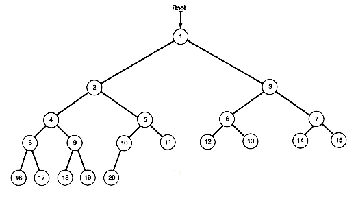
Figure 7.3 A Binary Tree
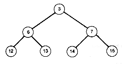
Figure 7.4 The Right Subtree of the Root of Figure 7.3

Figure 7.5 A Sparse Binary Tree
7.1.1 Depth versus Capacity*
n
 2d - 1
dmin =
 lg (n + 1)
 x indicates the smallest integer that equals or exceeds x. If n = 20, then dmin = lg 21 = 4.39 = 5; and if n = 31, then dmin = lg 32 =5. The binary tree corresponding to dmin may always be taken as a complete binary tree. Consequently, the depth of a complete binary tree will never exceed (lg n) + 1. This contrasts sharply with the depth of the sparsest binary tree with n nodes, which is n . For instance, if n is 1,000, the complete binary tree has a depth of only 10, while the sparsest has depth 1,000. This has important implications for how trees are constructed and for information retrieval, as shown in Chapter 9.
7.2: Trees of Records
7.2.1 Insertion and Deletion of Records in Binary Trees
p = avail();
setinfo(p,&value);
setleft(p,null);
setright(p,null);
setright(predecessor,p);

Figure 7.6 A Binary Tree T before and after the Insertion of C
q = right(predecessor);
p = avail();
setinfo(p,&value);
setleft(p,left(q));
setright(p,right(q));
setright(predecessor,p);
reclaim(q);
if(left(predecessor) == p)
setleft(predecessor,null);
else
1 otherwise
setright(predecessor, null);
1 set its predecessor's right pointer to null
7.2.2 Climbing Binary Trees
locust
oclsut
costul
7.2.3 Three Preorder Traversals of a Binary Tree
preorder(ptree)
/* Preorder traverses the
binary tree tree.
*/
binarytreepointer *ptree;
{binarytreepointer 1,r,setnull(),left(),right();
if(*ptree != setnull())
{process(ptree);
1 = left(*ptree);
preorder(&l);
r = right(*ptree);
preorder(&r);
}
}
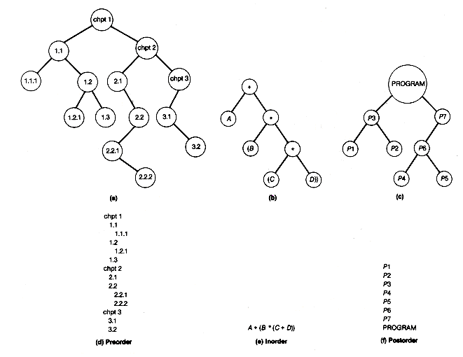
Figure 7.7 Trees for (a) a Table of Contents, (b) an Arithmetic Expression, and (c) Components of a Program. Order of Access to Nodes is (d) for Preorder Traversal of (a), (e) for Inorder Traversal of (b), and (f) for Postorder Traversal of (c)
preorder(ptree)
/* Preorder traverses the
binary tree tree.
*/
binarytreepointer *ptree;
{binarytreepointer p, null, setnull(), left(), right();
stack s;
null = setnull();
setstack(&s);
p = *ptree;
while ((p != null) || !empty(&s))
if (p != null)
{process (ptree,p);
push (right(p),&s);
p = left(p);
}
else
pop (&s,&p);
}
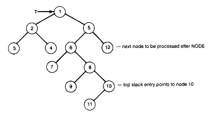
Figure 7.8 Node 5's Left Subtree Has Just Been Traversed
preorder(ptree)
/* Preorder traverses the
binary tree tree.
*/
binarytreepointer *ptree;
{binarytreepointer null,p,q,rightpointer;
binarytreepointer setnull(),left(),right(),item();
stack s;
null = setnull();
setstack(&s);
p = *ptree;
while((p != null) || !empty(&s))
if(p != null)
1 if there is a current node
{process(ptree,p);
if(left(p) != null)
{push(p,&s);
p = left(p);
}
else
{push(p,&s);
p = right(p);
}
}
else
1 otherwise
{do
{pop(&s,&q);
if (!empty(&s))
rightpointer = right(item(&s));
else
rightpointer = null;
}while(!empty(&s)&&(q==rightpointer));
if(q != rightpointer)
p = rightpointer;
}
}
7.3: Using the Traverse Functions for Binary Trees
process(ptree,p,ps)
/* Prints the number of terminal nodes in
binary tree tree when p points to the last
node in a preorder traverse of tree which
saves right pointers on stack s.
*/
binarytreepointer *ptree,p;
stack *ps;
{binarytreepointer null,setnull(),left(),right();
static int tncount;
null = setnull();
if(p == *ptree)
tncount = 0;
if((left(p) == null) && (right(p) == null))
{tncount++;
if(last (ps))
printf("\n The number of terminal nodes is %d",tncount);}
}
process(ptree,p,null,ps,value)
/* If p points to the first terminal node, encountered
in a preorder traversal of binary tree tree that saves
the path to the root on stack s, then replaces that node by
a new node whose info field is set to the contents of value.
*/
binarytreepointer *ptree,p,null;
stack *ps;
int value;
{binarytreepointer q,ptr,avail(),
left(),right();
if((left(p) == null)&&(right(p) == null)
{ptr = avail();
setinfo(ptr,&value);
setleft(ptr,null);
setright(ptr,null);
if(p != *ptree)
{q = item(ps);
if(left(q) == p)
setleft(q,ptr);
else
setright(q,ptr);
}
else
*ptree = ptr;
setstack(ps);
}
}
depth(tree)
/* Returns the depth of
the binary tree tree.
*/
binarytreepointer tree;
{binarytreepointer setnull(),left(),right();
if(tree == setnull())
return(0);
else
return(1 + max(depth(left(tree)),
depth(right(tree))));
}
7.4: Implementing Binary Trees
7.4.1 Sequential Representation

Figure 7.9 Sequential Representation of a Binary Tree
7.4.2 Linked Representation
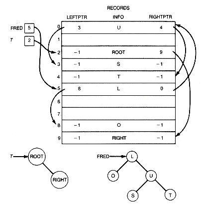
Figure 7.10 Linked Representation for Binary Trees with Records Stored in an Array
typedef struct
{whatever info;
int leftptr;
int rightptr;
}binarytreenode;
typedef int binarytreepointer;
# define MAX 50
typedef binarytreenode recordsarray[MAX];
recordsarray records;
typedef struct treenode
{whatever info;
struct treenode *leftptr;
struct treenode *rightptr;
}binarytreenode,*binarytreepointer;
1 indicates nonnull binary tree
3 data for the root;
11 both its subtrees are nonnull
6 data for the next record in preorder;
11 both its subtrees are nonnull1
12 data for the next record in preorder;
00 both its subtrees are null1
13 data for the next record in preorder;
00 both its subtrees are null
7 data for the next record in preorder;
00 both its subtrees are null
50 the new value
Reads the data for nodes of a binary tree, creates
the tree and prints how many terminal nodes it
has and its depth, reads the value for the new node,
replaces the first terminal node in preorder access
by the new node, and then prints all the final binary
tree's nodes, its terminal count, and its depth.
#include <stdio.h>
typedef struct treerecord
{int info;
struct treerecord *leftptr;
struct treerecord *rightptr;
}binarytreerecord,*binarytreepointer;
#define NULL 0
binarytreepointer left(p)
/* Returns a copy of the left
pointer of the node p points to.
*/
binarytreepointer p;
{return(p->leftptr);
}
binarytreepointer right(p)
/* Returns a copy of the right
pointer of the node p points to.
*/
binarytreepointer p;
{return(p->rightptr);
}
binarytreepointer setnull()
/* Returns a null pointer */
{return(NULL);
}
binarytreepointer avail()
/* Returns a pointer to storage
allocated for a new node.
*/
{return(malloc(sizeof(binarytreerecord)));
}
setinfo(p,pvalue)
/* Copies the contents of value
into the record p points to.
*/
binarytreepointer p;
int *pvalue;
{p->info = *pvalue;
}
setleft(p,q)
/* Copies q into the left pointer
of the record p points to.
*/
binarytreepointer p,q;
{p->leftptr = q;
}
setright(p,q)
/* Copies q into the right pointer
of the record p points to.
*/
binarytreepointer p,q;
{p->rightptr = q;
}
printnode(pl,ptr)
/* Prints the info field of the
record ptr points to.
*/
binarytreepointer *pl,ptr;
{printf("\n %d",ptr->info);}
main()
/* Reads the data for nodes of a binary tree, creates
the tree and prints how many terminal nodes it
has and its depth, reads the value for the new node,
replaces the first terminal node in preorder access
by the new node, and then prints all the final
binary tree's nodes, its terminal count, and its
depth.
*/
{int n,value;
binarytreepointer t,setnull(),avail();
printf("\n enter binarytree 0 for null tree 1\otherwise \n");
scanf("%d",&n);if (n == 0)
t = setnull();
else
{t = avail();
createtree(&t);
}
printtree(&t);
terminalcount(&t);
printf("\n The depth is %d",depth(t));printf("\n enter value ");scanf("%d",&value);replacefirstterminal(&t,value);
printtree(&t);
terminalcount(&t);
printf("\n The depth is %d",depth(t));}
createtree(ptree)
/* Read the data and create the binary tree tree. */
binarytreepointer *ptree;
{binarytreepointer l,r,setnull(),left(),right();
if (*ptree != setnull())
{createnode(ptree);
l = left(*ptree);
createtree(&l);
r = right(*ptree);
createtree(&r);
}
}
createnode(pptr)
/* Reads the data, and fills in the fields
of the node pointed to by ptr.
*/
binarytreepointer *pptr;
{int leftlink,rightlink,value;
binarytreepointer setnull(),avail();
printf("\n enter info \n");scanf("%d",&value);setinfo(*pptr,&value);
printf("\n enter enter left & right ptrs \n");scanf("%d %d",&leftlink,&rightlink);if (leftlink == 0)
setleft(*pptr,setnull());
else
setleft(*pptr,avail());
if (rightlink == 0)
setright(*pptr,setnull();
else
setright(*pptr,avail());
}
#define LIMIT 50
typedef binarytreepointer whatever;
typedef struct
{whatever stackarray[LIMIT];
int top;
}stack;
#define TRUE 1
#define FALSE 0
setstack(ps)
/* Sets the stack s to empty. */
stack *ps;
{(*ps).top = -1;
}
empty(ps)
/* Returns true only if stack s is empty.*/
stack *ps;
{return((*ps).top == -1);
}
push(value,ps)
/* Inserts value at the top of stack s. */
whatever value;
stack *ps;
{if ((*ps).top == (LIMIT - 1))
overflow(ps);
else
{(*ps).top = (*ps).top + 1;
(*ps).stackarray[(*ps).top] = value;
}
}
pop(ps,pvalue)
/* Removes the top entry of stack s
and copies its contents into value.
*/
stack *ps;
whatever *pvalue;
{if (empty(ps))
underflow(ps);
else
{*pvalue = (*ps).stackarray[(*ps).top];
(*ps).top = (*ps).top - 1;
}
}
whatever item(ps)
/* Returns a copy of the top entry on stack s. */
stack *ps;
{return((*ps).stackarray[(*ps).top]);
}
last(ps)
/* Returns true only if stack s
contains no non null pointers.
*/
stack *ps;
{int i,temp;
binarytreepointer null,setnull();
null = setnull();
temp = TRUE;
for (i=0;i<=(*ps).top;i++)
if ((*ps).stackarray[i] != null)
temp = FALSE;
return(temp);
}
overflow(ps)
/* Prints a message if the stack overflows. */
stack *ps;
{printf("\n stack overflow ");}
underflow(ps)
/* Prints a message if the stack underflows. */
stack *ps;
{printf("\n stack underflow ");}
printtree(ptree)
/* Prints the info field values of all
nodes of the binary tree tree.
*/
binarytreepointer *ptree;
{binarytreepointer null,p,q,rightpointer;
binarytreepointer setnull(),left(),right(),item();
stack s1;
null = setnull();
setstack(&s1);
p = *ptree;
while ((p != null) || !empty(&s1))
if (p != null)
{printnode(ptree,p);
if (left(p) != null)
{push(p,&s1);
p = left(p);
}
else
{push(p,&s1);
p = right(p);
}
}
else
{do
{pop(&s1,&q);
if (!empty(&s1))
rightpointer = right(item(&s1));
else
rightpointer = null;
}while(!empty(&s1) &&
(q == rightpointer));
if (q != rightpointer)
p = rightpointer;
}
}
terminalcount(ptree)
/* Prints the number of terminal nodes
in the binary tree tree.
*/
binarytreepointer *ptree;
{binarytreepointer p,null,setnull(),left(),right();
stack s2;
null = setnull();
setstack(&s2);
p = *ptree;
while ((p != null) || !empty(&s2))
if (p != null)
{updatetncount(ptree,p,&s2);
push(right(p),&s2);
p = left(p);
}
else
pop(&s2,&p);
}
updatetncount(pt,p,ps)
/* Prints the number of terminal nodes in
binary tree tree when p points to the last
node in a preorder traverse of tree which
saves right pointers on stack s.
*/
binarytreepointer *pt,p;
stack *ps;
{binarytreepointer null,setnull(),left(),right();
static int tncount;
null = setnull();
if (p == *pt)
tncount = O;
if ((left(p) == null) && (right(p) == null))
{tncount++;
if (last(ps))
printf("\n The number of terminal nodes\is %d",tncount);
}
}
replacefirstterminal(ptree,value)
/* Replaces the first terminal node, encountered
in a preorder traversal of binary tree tree, by a
new node with its info field set to the contents
of value.
*/
binarytreepointer *ptree;
int value;
{binarytreepointer null,p,q,rightpointer;
binarytreepointer setnull(),left(),right(),item();
stack s3;
null = setnull();
setstack(&s3);
p = *ptree;
while ((p != null) | | !empty(&s3))
if (p != null)
{replacenode(ptree,p,null,&s
 ,value);
if (left (p) != null)
{push(p,&s3);
p = left(p);
}
else
{push(p,&s3);
p = right(p);
}
}
else
{do
{pop(&s3,&q);
if (!empty(&s3))
rightpointer = right(item(&s3));
else
rightpointer = null;
}while (!empty(&s3) &&
(q == rightpointer));
if (q != rightpointer)
p = right pointer;
}
}
replacenode(ptree,p,null,ps,value)
/* If p points to the first terminal node, encountered
in a preorder traversal of binary tree tree that
saves the path to the root on stack s, then
replaces that node by a new node whose info field is
set to the contents of value.
*/
binarytreepointer *ptree,p,null;
stack *ps;
int value;
{binarytreepointer q,ptr,avail(),left(),right();
if ((left(p) == null) && (right(p) == null))
{ptr = avail();
setinfo(ptr,&value);
setleft(ptr,null);
setright(ptr,null);
if (p != *ptree)
{q = item(ps);
if (left(q) == p)
setleft(q,ptr);
else
setright(q,ptr);
}
else
*ptree = ptr;
setstack(ps);
}
}
depth(tree)
/* Returns the depth of the binary tree tree. */
binarytreepointer tree;
{binarytreepointer setnull(),left(),right();
if (tree == setnull())
return(0);
else
return(1 + max(depth(left(tree)),
depth(right(tree))));
}
max(i,j)
/* Returns the maximum of i and j. */
int i,j;
{if (i >= j)
return(i);
else
return(j);
}
7.4.3 List-structure Representation
7.5: Trees
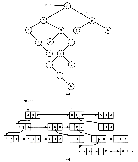
Figure 7.11 (a) List-structure Representation of (b) a Binary Tree
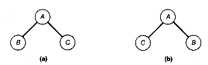
Figure 7.12 Two Distinct Binary Trees or One General Tree
7.5.1 Implementing Trees as Binary Trees
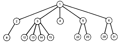
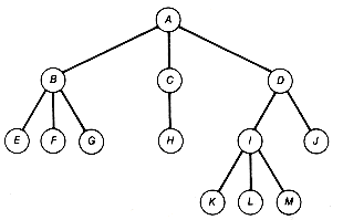
(a) Initial Tree
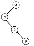
(b) Binary Tree for Nodes A - D
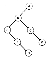
(c) Binary Tree for Nodes A - G
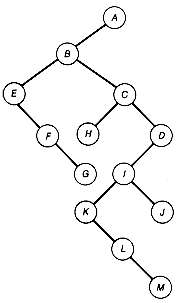
(d) Final Binary Tree
Figure 7.13 Representation of a General Tree as a Binary Tree
7.6: Traversals of Trees
7.6.1 Obtaining the Binary Tree for a Tree
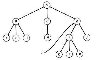
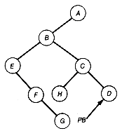
Figure 7.14 Binary Tree BT Generated from General Tree T

Figure 7.15 Generation of Binary Tree BT from an Ordered Tree T
7.6.2 Backtracking: The n-queens Problem
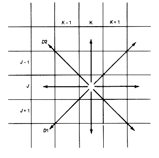
Figure 7.16 A Partial Chessboard Represented as a Two-Dimensional Array, BOARD
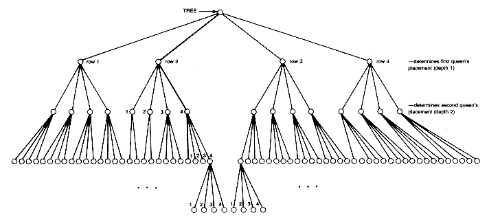
Figure 7.17 Tree for the Four-queens Problem
7.6.3 Depth-first
# include <stdio.h>
main()
/* Reads in n and prints all solutions
to the n-queens problem.
*/
{int n;
printf("\n n = ?");scanf("%d",&n);queens(n);
}
#define NLIMIT 20
typedef int rowcheck[NLIMIT];
typedef int diagonalcheck1[2*NLIMIT-1];
typedef int diagonalcheck2[2*NLIMIT-1];
#define SLIMIT 20
typedef int whatever;
typedef struct
{whatever stackarray[SLIMIT--1];
int top;
}stack;
setstack(ps)
/* Sets stack s to empty. */
stack *ps;
{(*ps).top = --1;
}
empty(ps)
/* Returns true only if stack s is empty. */
stack *ps;
{return((*ps).top == -1);
}
push(value,ps)
/* Inserts contents of value as
the top entry on stack s.
/*
whatever value;
stack *ps;
{if((*ps).top == (SLIMIT-1))
overflow(ps);
else
{(*ps).top = (*ps).top + 1;
(*ps).stackarray[(*ps).top] = value;
}
}
pop(ps,pvalue)
/* Removes the top entry of stack s
and copies its contents into value.
*/
stack *ps;
whatever *pvalue;
{if(empty(ps))
underflow(ps);
else
{*pvalue = (*ps).stackarray[(*ps).top];
(*ps).top = (*ps).top - 1;
}
}
whatever item(i,ps)
/* Returns a copy of the ith
entry in stack s. When i is
zero it returns a copy of
the top entry.
*/
stack *ps;
{return((*ps).stackarray[(*ps).top-i]);
}
overflow(ps)
/* Prints a message if the stack overflows. */
stack *ps;
{printf("\n stack overflow ");}
underflow(ps)
/* Prints a message if the stack underflows. */
stack *ps;
{printf("\n stack underflow ");}
queens(n)
1 a backtracking preorder traversal
/* Prints all solutions to the n-queens problem */
int n;
{stack s;
#define TRUE 1
#define FALSE 0
int i,row,col,found;
rowcheck r;
3 r, d1, and d2 will contain the board configuration
diagonalcheck1 d1;
diagonalcheck2 d2;
col = 1;
2 col and row determine the next placement attempt
row = 1;
for(i=0;i<=n-1;i++)
r[i] = TRUE;
for(i=0;i<=2*n-2;i++)
d1[i] = TRUE;
for(i=0;i<=2*n-2;i++)
d2[i] = TRUE;
found = FALSE;
setstack(&s);
while(((col < n+1)&&(row < n+1)) || !empty(&s))
if((col < n+1)&&(row < n+1))
if(feasible(row,col,r,d1,d2,n))
{process(row,col,&found,&s,n);
push(row,&s);
r[row-1] = FALSE;
d1[row+col-2] = FALSE;
d2[row-col+n-1] = FALSE;
col = col + 1;
row = 1;
}
else
row = row + 1;
else
{pop(&s,&row);
col = col - 1;
r[row-1] = TRUE
d1[row+col-2] = TRUE;
d2[row-col+n-1] = TRUE;
row = row + 1;
}
if(!found)
printf("\n NO SOLUTIONS");}
feasible(row,col,r,d1,d2,n)
/* Returns true only if the placement of the
next queen in position col,row does not
allow any queen to take another under
the current board configuration given
by r,d1,d2.
*/
int row,col, n;
rowcheck r;
diagonalcheck1 d1;
diagonalcheck2 d2;
{return(r[row-1]&&d1[row+col-2]&&d2[row-col+n-1]);
}
process(row,col,pfound,ps,n)
/* If the partial solution is a complete
solution then it is printed and
found is set to true.
*/
int row,col,*pfound,n;
stack *ps;
{int i;
whatever item();
if(col == n)
{for(i=n-1;i>=1;i--)
printf("\n COL %d ROW is %d----",n-1,item(i-1,ps));
printf("\n COL %d ROW is %d----\n",n,row);
*pfound = TRUE;
}
}
 4. For the curious, the number of solutions for n up to 15 are:
 N 4 5 6 7 8 9 10
Solutions 2 10 4 40 92 352 724
N 11 12 13 14 15
Solutions 2,680 14,200 73,712 365,596 2,279,184
7.6.4 Breadth-first
7.6.5 Branch and Bound
7.7: More on Recursion, Trees, and Stacks
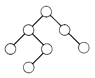
(a) Balanced
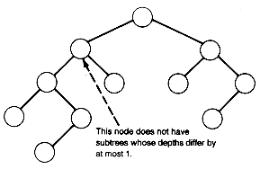
(b) Unbalanced
Figure 7.18 Balanced and Unbalanced Binary Trees
7.7.1 Balanced Binary Trees

Figure 7.19 A Fibonacci Tree of Depth 4
F0 = 0, F1 = 1,
Fn = Fn-1 + Fn-2 for n > 1
fibonaccitree (d, ptree)
/* Creates a Fibonacci tree, tree, of depth d. */
int d;
binarytreepointer *ptree;
{binarytreepointer tl, tr, avail ( );
*ptree = avail ( );
if (d == 0)
*ptree = NULL;
else if (d == 1)
{records [*ptree].leftptr = NULL;
records [*ptree].rightptr = NULL;
}
else
{fibonaccitree (d-2,&tl);
records [*ptree].leftptr = tl;
fibonaccitree (d-1,&tr);
records [*ptree].rightptr = tr;
}
}
fibonaccitree(d,ptree)
/* Creates a Fibonacci tree, tree, of depth d. */
int d;
binarytreepointer *ptree;
{binarytreepointer tl, tr;
*ptree = malloc (sizeof(binarytreerecord));
if (d == 0)
*ptree = NULL;
else if (d == 1)
{(*ptree)->leftptr = NULL;
(*ptree)->rightptr = NULL;
}
else
{fibonaccitree (d-2, &tl);
(*ptree)->leftptr = tl;
fibonaccitree (d-1, &tr);
(*ptree)->rightptr = tr;
}
}
fibonaccitree(d,ptree)
/* Creates a Fibonacci tree, tree, of depth d. */
int d;
binarytreepointer *ptree;
{binarytreepointer null,tl,tr,avail( ),setnull( );
null = setnull( );
*ptree = avail( );
if (d == 0)
*ptree = null;
else if (d == 1)
{setleft(*ptree, null);
setright(*ptree, null);
}
else
{fibonaccitree(d-2,&tl);
setleft(*ptree, tl);
fibonaccitree(d-1,&tr);
setleft(*ptree, tr);
}
}
7.7.2 Trading Storage for Time
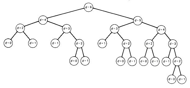
Figure 7.20 Execution Tree for Depth d = 6
 d), where = (1 +
  )/2.* This is because 2 can be constructed even if only Fibonacci trees of depth d - 2 and d - 1 are known. All that is necessary is to create a root node and append the tree of depth d - 2 as its left subtree and the tree of depth d - 1 as its right subtree. Consequently, the Fibonacci tree of depth d can be obtained by constructing the trees for depth 0, 1, 2 . . . , d in turn, while retaining only the lastest two. This gives the nonrecursive solution:
Exercises

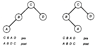
5
8 L 0
-1 O -1
3 U 4
-1 S -1
-1 T -1
leftptr info rightptr
1 0 R 0
2 3 W 4
3 5 R 0
sample 7 4 0 C 0
5 4 E 6
6 0 T 0
7 10 C 3
8 6 A 3
9 1 B 4
10 1 O 0
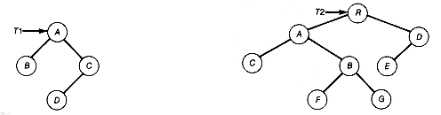
(a) Input
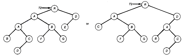
(b) Output


check (t1,t2)
binarytreepointer t1,t2;
{binarytreepointer null,setnull();
null = setnull();
if(((t1 == null) && (t2 == null)) || ((t1 != null)
&& (t2 != null)))
return(check(t1->leftptr,t2->leftptr)
&& check(t1->rightptr,t2->rightptr));
else
return (FALSE);
}
b(0) = 1
b(n) = b(0) X b(n - 1) + b(1) X b(n - 2) + b(2)b(n - 3) + . . .
+ b(n - 1) x b(0) n > 0
Suggested Assignments