


In languages such as C, arrays are static data structures. They do not change size or shape during the execution of a program. Chains, however, do change size, though they don't change shape. They are dynamic. List-structures, more complex lists, and binary and general trees can change both size and shape and thus are also dynamic data structures. The basic distinction between static and dynamic data structures relates to whether a fixed amount of memory is allocated in advance of program execution. Static structures can have a fixed amount of memory allocated for their sole use prior to program execution. For dynamic structures, the amount of memory required is not known in advance and thus cannot be allocated in this way.
In FORTRAN and COBOL, the total amount of storage needed by the variables of a program is known by the compiler and can be set aside before program execution. This means that a fixed amount of storage is allocated to variables for the entire execution of the program. This is not done in C, which is more versatile. It uses both static and dynamic storage allocation. Some storage is allocated for the entire execution of the program, while other storage is allocated when needed and is reused when no longer needed. This requires storage management during program execution. Dynamic structures such as lists and trees need even more complex storage management during program execution.
Consider a program that maintains a data base of stock portfolios for the clients of a brokerage house. Suppose each client's stocks are kept in a binary search tree ordered by stock name, with each node of the tree represented as a record containing information about the stock. It is not possible to predict in advance how much storage is needed, since how many stocks each client will buy is not known. Experience may show that all clients' stocks will never number more than 2,000, but the distribution of these stocks among the clients varies throughout the year. Thus it will be necessary to have storage available for 2,000 records. At a given moment this storage will be distributed among the clients' binary search trees. Whenever a stock is sold for one client, its storage must be deleted from that client's tree. It may be needed later to store the record of a stock just bought for another client. This allocation and reclaiming of record storage during program execution requires dynamic storage management. Some languages, such as C, provide needed storage management. Others do not, so the programmer must provide it.
This chapter discusses the fundamentals of storage management techniques. It offers insight into how programming languages manage storage and provides a better appreciation of the pitfalls that lie below the surface features of a language. Such insight is especially important when the programmer employs complex data structures that share storage.
You have already seen in Chapter 3 how the simple case of fixed-length records with no sharing might be handled. Problems arise when records have variable lengths and when data structures share memory. The remedies for these problems involve the creation and processing of data structures tailored to these needs. Sophisticated traversal algorithms have been developed to conserve storage. They are introduced here for three reasons. First, they are essential for the implementation of those data structures. Second, they are interesting in themselves. Finally, they serve as a good example of the use of data abstraction.
Although storage management is viewed here from the perspective of a single program's needs, these same techniques are employed by operating systems to deal with the allocation and reclamation of storage for a group of active programs.
In some problems, an upper bound on the problem size is not known in advance. One way to deal with this situation is to pick a reasonably large size and declare static data structures of this size. If the problem's memory requirement exceeds this size, an error message may be printed. When the number of available memory elements is fixed, there will generally be some problem size for which programs fail. However, it is possible that the program uses several data structures. During execution, when one data structure is large the others may be small, so that the total amount of storage required for all the structures may actually be available at all times. With static data structures, where memory is allocated and remains dedicated to a particular structure, storage must be allocated to accommodate the worst case. The worst case calls for the sum of the maximum storages needed for each data structure of the program. If, instead, the available memory can be used for the data structure that currently requires it and reclaimed for later use when that structure no longer needs it, then larger problems can be solved. This point is illustrated in the following examples.
Example 13.1
The lists array used to store successor records for the topological sort of Chapter 11 allows all successor lists to share storage. No storage is dedicated to any individual list. As long as the total number of successors on all lists does not exceed the length of lists, the program will execute correctly. This contrasts with the alternate collection of n arrays discussed in Section 11.6. With the latter approach, storage is dedicated to each list; although twice as many total successors may be accommodated, no list can contain more than its dedicated amount.
Example 13.2
Suppose five stacks are each implemented, as in Chapter 4, using static array structures, each with a maximum size of 5,000 elements. This requires 25,000 total memory locations. However, if the number of entries in all the stacks at any one time never exceeds 10,000, proper sharing of storage would allow a reduction of up to 15,000 in the amount of storage needed.
Example 13.3
A program can store, in linked representation, a number of binary trees that must be traversed using stacks. If the trees must be stored and traversed simultaneously, it is possible that available storage for the records of the tree nodes and for the entries of the stacks will not be sufficient for the worst case. However, if the available storage can be shared, so that it is used for tree records or for stack entries when needed, then the program might execute correctly.
In Example 13.1, the records sharing storage all have the same size. In Example 13.2, the five stacks can all store records of the same size, or they can store records of different lengths. Example 13.3 needs shared storage for records, which may or may not be of the same length for each binary tree, and for stack entries. Normally the record lengths would be significantly greater than that of the stack entries. One fundamental distinction between storage management techniques involves whether or not the storage allocated will all be the same size. When dealing with the fixed-size case, it is convenient to use the techniques for storage allocation and storage reclamation, discussed in Chapter 3, which involve a list of available space. When dealing with more general data structures or with variable-size records, additional complications arise.
As one or more programs execute, they may require storage for the creation of new records, which typically are to be inserted into dynamic data structures. How can a fixed amount of storage that is made available for the creation of these records be managed efficiently?
The records, or more generally, the components of dynamic data structures, are referred to as nodes. The region of memory consisting of contiguous elements that is dedicated to the storage of these nodes is called the heap or dynamic memory. We will use the term heap in the further discussion. In the heap all nodes need not be the same length, and nodes may appear as part of more than one data structure. Associated with each node is a length field, indicating the size of the node (that is, the number of memory elements it uses). If all nodes were the same size, there would be no need to store size information within each node. All dynamic data structures reside in the heap. At all times, the heap may contain three kinds of nodes:
Nodes that are in use because they appear in dynamic data structures
Nodes that are not in use and appear in no dynamic data structure but are on the current list of available space
Nodes that are not in use because they are in no dynamic data structure but are not on the list of available space
Nodes on the list of available space are said to be known. Nodes that are available but not on the list of available space are called garbage. All heads (names) of dynamic data structures, which point to their first records, are outside the heap and are kept track of in some way. This means that at all times the program knows what dynamic data structures are in existence, since their names are known.
Example 13.4
Suppose av, 1, and t are, respectively, the heads of the available space list, a list, and a binary tree. A heap containing these dynamic data structures may be visualized as in Figure 13.1. Each node has been labeled to indicate its current status:
1--in use since the node appears on l or t
2--not in use but on the available space list
3--not in use and not on the available space list, hence garbage
Storage allocation now involves three tasks:
1. Decide which node on the list of available space will be made available when a request for creation of a node is made.
2. Delete that node from the list of available space.
3. Set a pointer value to point to the node.
An avail-like function, discussed in Chapter 3, will perform these three tasks.
When dealing with variable-size records, which is the usual situation, storage management is complex because of fragmentation. The fragmentation problem is as follows. When all records being allocated dynamically are the same size, then as long as unused storage finds its way to the list of available space, it can be reused. However, it is possible with variable-size records that storage for a large record is needed but is not immediately in existence. Suppose each available block of consecutive elements of storage is kept on the list of available space as an individual record, with a field of each record used to store its length. It is possible for records of length 10, 15, 3, 20, and 45 to appear on the list when a record of length 65 must be created, but no individual record is large enough to be allocated for it. However, a total of 93 elements is unused. This is the external fragmentation problem. Enough storage is unused to satisfy the need, but no record currently on the list of available space is, by itself, large enough to be used. The problem may be resolved by invoking a compaction procedure, which moves the field values in used nodes to contiguous elements of memory at one end of the heap. All unused elements then also become contiguous and can represent a node large enough that the needed storage can be taken.
Example 13.5
Suppose the compaction procedure is applied to the heap of Example 13.4, which was illustrated in Figure 13.1. The result may be visualized as in Figure 13.2.
Compaction, like garbage collection, is a time-consuming process that the programmer or computer system should only invoke infrequently. To overcome this, it is possible to organize the list of available space in an attempt to minimize fragmentation and thus the need for compaction. However, in limiting fragmentation the program should not spend too much computer time determining which node to allocate each time a request is made. Organizing the list of available space and using a reasonable policy to select the node to be allocated helps to reduce fragmentation. However, additional time is required to search the list to select the node to be allocated and to place a reclaimed node in proper position on the list to maintain its organization.
Fragmentation can also be reduced by creating larger nodes, by adding the freed storage to storage adjacent to it that is already free. This process is called coalescing. These policies and ways of organizing must be addressed by designers of compilers or operating systems and by programmers when they create storage management schemes for their own use.
Recall that the more structured or organized the data, the faster the access to required information. At the same time a price must be paid to maintain the organization. The primary considerations for a storage management scheme are the time to satisfy a request for a new node, the time to insert a node on the list of available space, the storage utilization, and the likelihood of satisfying a request. How well these characteristics turn out for a particular storage management scheme depends on the sequence of requests and returns. Mathematical analysis is generally not possible, and simulation must be used to evaluate different schemes. To provide some idea of the trade-offs and possibilities, three fundamental organizations for the available space list and appropriate allocation and reclamation policies are presented next.
The simplest organization for the list of available space is a two-way circular list, with nodes kept in arbitrary order, in order by size, or in order by actual memory address. Two-way lists are convenient for making insertions and deletions. They allow the list to be traversed starting from any list record, and in either direction. A request for a node of size l then requires a traversal of the list, starting from some initial node.
Two simple policies for selection of the list node to be deleted to satisfy a request are first-fit and best-fit. First-fit selects the first node encountered whose size is sufficient. Best-fit does a complete traversal and selects that node of smallest size that is sufficient to satisfy the request. Of course, if an exact fit is found, the traversal need not continue. For both policies, any leftover storage is retained as a node on the list.
When a node is returned to the list, its neighbors (in terms of storage addresses) are coalesced with it if free, and the resultant node properly inserted on the list. All nodes require tag and size fields, with the list nodes also needing backward and forward link fields. The tag field distinguishes nodes in use from those not in use, depending on which of two values it contains.
Allowing the starting node to circulate around the list, always being set to the successor of the deleted (or truncated) node, typically improves performance.This circulation provides time for the smaller nodes left behind it to coalesce so that, by the next time around, larger nodes have been formed.
Intuitively, spending more time fitting the size of the selected node to the size of the requested node should cut down on fragmentation effects. Surprisingly, this need not always happen, but it is the normal situation.
Another organization, called the buddy system, provides faster request and return time responses than two-way circular lists. The buddy system requires the heap to be of length 2m for some integer m, occupying addresses 0 to 2m - 1. Over time, the heap is split into nodes of varying lengths. These lengths are constrained to be powers of 2, and nodes are kept on separate lists, each list containing nodes of a specific length. An array a of length m contains the heads of these lists, so a[k] points to the first node on the list corresponding to length 2k. Initially, a[m] points to the first address of the heap; all other array entries are null, since all other lists are empty.
To satisfy a request for a node of length n, k is set to
During this iterated splitting process, each time a node is split, it is split into two special nodes called buddies. Buddies bear a unique relation to each other. Only buddies are allowed to coalesce. Although this can result in unused nodes being contiguous but not coalescing because they are not buddies, it is a rare occurrence. This restriction allows very fast coalescing of buddies, as will be shown.
When a node is to be returned to the list of available space (a misnomer now), its buddy is first checked to see if it is not in use and, if it is not, the buddies are coalesced. This node is, in turn, coalesced with its buddy when possible, and so on, until no further coalescing is possible. This coalescing process is the reverse of the splitting process that created the buddies in the first place.
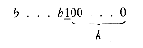
At this point you must be wondering how a node's buddy is found. The scheme ensures that it may be done quickly because a node of size 2k with starting address
has as its buddy a node of size 2k with starting address
In general, given the address of a node of size 2k to be returned, its (k + 1)th bit (addresses are expressed in binary notation) is changed from 1 to 0 or 0 to 1, and the result is the address of its buddy. A tag field is used to indicate whether or not a node is in use.
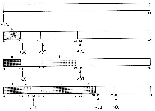
Example 13.6
How does the buddy system respond when m is 6 and a sequence of requests is made for nodes of size 8, 16, 4, and 6?
The sequence of memory configurations is as shown in Figure 13.3(a). lf the node of length 16 is now returned, the configuration becomes as shown in Figure13.3(b)
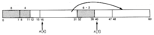
A[4] is now the head of a list with two nodes, each of length 16. The released node of length 16 starting at address 16 (10000 in binary) has the node of length 16 starting at address 0 (00000 in binary) as its buddy. Since it is not free, it cannot coalesce with it. Neither can it coalesce with the node of length 4 starting at address 12, since that node is not its buddy.
The distribution of nodes can be mirrored by a binary tree. This tree is a kind of derivation tree for nodes currently in existence and expands and contracts as nodes are split and coalesced. The tree shown in Figure 13.4 reflects the configuration for Example 13.6 before the node of length 16 is returned.
Buddies appear as successors of the same parent. Thus [12, 15] and [16, 31], although contiguous in memory, are not buddies and therefore may not be coalesced.
With the buddy system, lists are never actually traversed to find storage to allocate, although time is spent finding the proper list from which to take the storage. The result is quick response to requests and returns. However, in contrast to two-way lists, this scheme produces significant internal fragmentation. Internal fragmentation occurs when allocated nodes are larger than requested, resulting in wasted storage residing within a node. This is one of the drawbacks of the buddy system. Studies have been done on similar schemes that allow a greater variety of node sizes to appear. They also tend to be fast and to reduce storage loss due to internal fragmentation.
At this point each of the two approaches, circular lists and buddy systems, seems to solve half the problem. Circular lists using the best-fit method utilize storage very efficiently, causing little internal fragmentation. Buddy systems produce significant internal fragmentation but offer fast allocation by narrowly focusing the search for a proper size node. The question is whether it is possible to achieve good storage utilization and allocation time by combining their features. As you would guess, it is. It can be done by using the appropriate structures. The means to do it is called the indexing approach. The indexing approach breaks up the list of available space into collections of two-way circular lists. Each of these circular lists contains nodes of just one size. Each node on the circular list represents a block of consecutive memory locations available for the storage of a record of the size of the node. Assuming that requests for nodes of sizes (say, 1 to 4) are very frequent, an array a contains pointers to each of the four lists corresponding to these sizes. The last array entry contains a pointer to an AVL tree. The nodes of this tree are circular lists, each list corresponding to nodes of specific size that are requested much less frequently. Thus a[2] contains a pointer to a circular list containing four blocks or nodes, each of size 2. In the AVL tree pointed to by a[5], the root node is a circular list containing three blocks of size 10. The tree is ordered on the basis of node sizes. A typical configuration might be as shown in Figure 13.5.
In this way, a specific request for a node of length less than 5 can be quickly satisfied if the exact matching list is not empty. If it is empty, the next nonempty greater-size list can be used, with one of its nodes truncated to satisfy the request. Any leftover is inserted on the appropriate list. For instance, with the situation of Figure 13.5, a request for a node of size 3 will be satisfied by deleting a node of size 4 from the list pointed to by a[4]. This node will be split into a node of size 3 to satisfy the request, and the leftover node of size 1 inserted on the list pointed to by a[1]. In the infrequent case when the requested node size is 5 or greater, the AVL tree must be searched similarly. It is clear that this scheme can cause internal fragmentation, but the search times should be fast on the average. In fact the indexing approach is a compromise. It is not as fast as the buddy system but faster than simple circular lists. Likewise, the fragmentation is less than with the buddy system but more than with simple circular lists.
Thus choosing the appropriate scheme of storage management is a difficult task. It requires insight into the kind of request and return distribution involved in a given application. In the worst case all schemes may fail miserably. Intuitively, good performance should result when the distribution of node sizes on the list of available space reflects the distribution of requests and returns. In turn, this distribution should be reflected in the distribution of node sizes actually in use. This is analogous to the situation mentioned in Chapter 12 for the distribution of letters in printer's boxes. The distribution of letter requests is reflected in actual text, and the printer's ordering policy for letters should have caused the contents of the letter boxes to reflect this distribution.
The three techniques considered in this section, and other techniques, are compared extensively in Knuth [1973a] and Standish [1980]. See also Tremblay and Sorenson [1984].
When components of data structures are identical and require significant amounts of storage, it is only natural to attempt to avoid component replication. This means that identical components will all share the same storage, so references to each will always be to the same place. As an example, consider Figure 13.6. The two list-structures ls1 and ls2 share a common sublist. As a result, p1, p3, and p4 point to the shared sublist.
As usual, what we gain in one area we pay for in another. Here, storage is saved, but the price is paid in more complex processing. In particular, suppose the sublist pointed to by p3 is to be deleted from ls2 by setting p3 to null. Since p1 and p4 still point to it, it is not valid to return its records' storage to the list of available space, as would be the case without sharing. Deciding when and how to reclaim deleted records or sublists by insertion on the list of available space requires more sophisticated reclamation algorithms than those of Chapter 3.
Saying that a node or component of a data structure is to be reclaimed for use means that the storage used for its records is to become known to the avail function. That is, the storage no longer needed by its records is to be inserted on the list of available space. There are two basic methods of reclaiming released nodes, garbage collection and reference counters. Other methods are essentially combinations of these. These methods are the two extremes with respect to the time at which storage is reclaimed. Garbage collection does not make storage available for reuse until it is needed, putting off reclamation as long as possible. Reference counters make storage available for reuse as soon as it actually becomes reclaimable.
The garbage collection method of reclamation is used when the available space list is empty or when the amount of storage that is known to avail becomes less than some given amount. Until that time, whenever a sublist is to be deleted from a data structure, the deletion is accomplished by updating appropriate pointers, but the storage vacated by the sublist's deletion is not made known. Initially, all records are assumed to be unmarked. The garbage collection routine works by traversing each data structure that is in use and "marking" each one of its records as being in use.
To accomplish this properly, the garbage collector program must know the names of all data structures in use. We have assumed that these are accessible through variables outside the heap. After marking, every record of the heap that is not marked will be made known (that is, placed on the available space list). Every record that is marked will be reset to unmarked so that the garbage collector will work properly on its next call. The marking phase of the garbage collector works by traversing all data structures in use. Thus marking routines generally take execution time proportional to the number of records in use and are therefore slow. Similarly, the collection routine, which inserts the unmarked records on the list of available space, takes time proportional to the heap size.
Example 13.7
Apply garbage collection to the heap of Example 13.4.
In the marking phase, the garbage collection would traverse l and t, marking all their nodes. The collection phase would then traverse the heap and collect all unmarked nodes on the available space list. Assuming the garbage collector recognizes when two unmarked nodes are adjacent and combines them into a larger node, the resultant heap would appear as shown in Figure 13.7. A better approach might be to garbage collect and compact together, thus producing an available list consisting of one large block, reducing fragmentation.
The reference counter method assumes that the first record of every sublist in use has information giving the number of pointers that point to it. This number is called the reference count of the sublist. The pointers can be stored in the name variables or in sublist fields of complex records. A "smart" header record may be used for this purpose. It is assumed here that only sublists may be shared. Each time a new pointer refers to a sublist, the reference count of the sublist must be increased by 1. Each time a pointer that refers to a sublist is changed so that it no longer points to that sublist, the reference count of the sublist must be decreased by 1. After a decrease that leaves the reference count at zero, the storage for records of the sublist may be made known. Again, a data structure traversal may be used to determine which storage elements are to be made known. No traversal algorithm has been given in this text for data structures that allow sublist sharing. Such algorithms differ from the list-structure traversal algorithm because of the possibility of looping or revisiting records. As an exercise you should modify the list-structure traversals of Chapter 6 to work for this more general case. The idea is to mark each accessed record and make sure that marked records are not revisited.
Deletion of a sublist whose reference count has become zero is similar to the traversal of successor lists for an object that has been removed from the bag in the topological sort algorithm. The sublist must be traversed and, in addition to the storage for all records being inserted on the list of available space, each sublist pointed to by a record must have its reference count decremented by 1.
Example 13.8
Associate reference counts with the first record of each of the sublists of Figure 13.6. The list-structures with associated reference counts would appear as shown in Figure 13.8.
Suppose p1 is set to null. The reference count of its sublist would be reduced to 2. Since it has not gone to zero, no storage is available for reclamation. If p6 is then set to null, the reference count of its sublist would be reduced to 0. Its storage could be reclaimed. This would require that p3's sublist have its reference count reduced by 1. The result would be as shown in Figure 13.8(b).
A problem can occur with the reference counter method whenever loops appear, as demonstrated in the following example.
Example 13.9
Consider the loop in ls1 of Figure 13.9. What happens when p1, p2, and p3 of Figure 13.6 no longer reference the sublist? Then this sublist has no variables referencing it. It cannot be accessed, since we do not know where it is. It is serving no useful purpose, yet its storage was not reclaimed, since the reference count of records 1 and 2 never went to zero. This problem is analogous to the existence of loops in the input for a topological sort. Such unused storage, or garbage, can accumulate and clog the memory.
It is possible to share individual records as well as sublists. In this case, garbage collection will still work, as will the reference counter method. Now, however, the individual records (not just the sublists) must have reference counters associated with them, requiring additional storage and updating overhead. Loops may cause the same problems for shared records as for shared sublists .
There is a spectrum of reclamation techniques, but the two basic underlying approaches are garbage collection and reference counters. Garbage collection represents one extreme. Nodes that are no longer needed in a dynamic data structure are deleted from the structure, thus becoming garbage. They are not returned at that time to the list of available space, even though they are then reusable. Reference counters, at the other extreme, return such unused nodes to the list of available space as soon as possible, when their reference counters become zero. These methods of reclamation are done implicitly by the programming language in conjunction with the operating system.
In addition, programmer control allows the programmer to use commands signaling that nodes are no longer needed by a dynamic data structure. The nodes may then be returned to the list of available space directly, left for garbage collection, or, if reference counters are used, their reference counts will be decremented and tested for possible return to the list of available space. In C the standard library function free can be used for such signaling.
In the design of a specific reclamation system, a number of trade-offs are possible. For example, reference counters require additional storage and additional time to increment, decrement, or test when insertions and deletions occur. However, they do not always work. The reason is that garbage can accumulate when loops are present in the dynamic data structures (as in Example 13.9). If the amount of garbage generated in this way is significant, it can limit the size of the problem that can be solved. Still, reference counters allow the reclamation process to be spread over time. Garbage collection, in contrast, occasionally requires a relatively large block of time. Garbage collection is a more complex technique, involving more sophisticated algorithms. Recall that when garbage collection is invoked, even though many available nodes may exist, they are not known. It is not possible simply to look at a node of the heap to determine if it is in use.
To summarize, garbage collection works in two phases. The first phase, or marking phase, requires the traversal of all dynamic data structures in existence. Recall that the heads of such structures are assumed to be known. Initially, whether in use or not, every node has a field that is marked "unused." As each node of a dynamic data structure is accessed in the traversal, it is marked "used." When the marking phase is completed, the heap then consists of nodes that are marked "unused" and nodes that are marked "used." Consequently, it is now possible to look at a node and determine its status. The second phase, or collection phase, involves a traversal through the nodes of the heap. Each node marked "unused" is inserted on the list of available space. Each node marked "used" is merely marked "unused" so that the garbage collector will work correctly the next time it is invoked.
The marking algorithms known are quite elegant. The traversal of the dynamic data structures cannot simply use a stack, since no nodes are known in which to implement the stack. Instead, these algorithms allow the traversals to be accomplished by using tag fields, usually one bit, associated with each node. It is even possible to do the traversals with no tag fields, with a fixed amount of additional storage required. Of course, if we had an infinite amount of storage available, no reclamation would be necessary. Storage management would be trivial! The next section features three traversal algorithms for use in phase I of the garbage collector, or in other applications where storage is at a premium. See Pratt [1975] for more on storage management. The algorithms to be discussed next and generalizations are also given in Standish [1980].
Garbage collection routines require the traversal of dynamic data structures that are more general than binary trees, such as list-structures and more complex lists. Algorithms for their traversal are generalizations of those we consider. For increased clarity, we will restrict our discussion to binary tree traversals and present three techniques that do not use extra storage for a stack.
These algorithms may be written assuming a particular binary tree implementation, such as arrays or pointer variables. Instead, to emphasize data abstraction and functional modularity, the following function, which is independent of the tree implementation, has been chosen. The function is a preorder traversal saving the path from the root on the stack.
For each traversal, the basic concept is described. Then the appropriate implementation for the routines of the procedure is described.
Consider the binary tree of Figure 13.10, and suppose node.p has just been processed during the traversal using the preorder procedure. The stack will contain pointers p1, p2, p3, p4, p5, p6, and p7. At this point, the traversal of the left subtree of node.p4 has been completed. The purpose of the nextsubtree(&s,&p) function in the preorder traversal algorithms is to find node.p4, to allow the traversal to pick up at its right subtree. In general, whenever the stack is not empty, a null p value signifies the completion of the traversal of the left subtree of some node. The traversal must then pick up at that node's right subtree. There may be more than one such node; it is the most recent that must be found. The stack allows this node, and its right subtree, to be found conveniently. Nextsubtree(&s,&p) is called after the terminal node pointed to by p has been processed. It finds the nonnull right subtree that must be traversed next, returns a pointer to it, and updates the stack to reflect the path from that subtree's root to the root of the tree. If no such nonnull right subtree exists, then it returns a null value. Each of the tree traversals we now consider actually uses stack information, but it is, in effect, stored in the tree, eliminating the requirement for additional stack storage. The preorder procedure treats the tree as a data abstraction, so it is independent of the tree implementation.
A threaded tree implementation of the preorder traversal procedure is shown in Figure 13.11. It resulted from the replacement of the null left and right pointer field values of each node t by a pointer to the predecessor and to the successor, respectively, of that node in an inorder traversal of t. These pointers are called threads. The "leftmost" node of t does not have a predecessor, and the "rightmost" node of t does not have a successor. Their left and right null pointers, respectively, are left unchanged and are not considered threads. We assume that a field is associated with each node to indicate whether the node contains threads in its left link field, in its right link field, in both, or in neither.
To preorder traverse threaded trees, proceed as before, but whenever a node with threads is reached, follow its right pointer. This pointer leads directly to the node whose right subtree must then be preorder traversed. Notice, for example, that the right thread of node.p points to node.p4. The traversal is complete when a null right thread is encountered. Threaded trees may also be easily inorder and postorder traversed.
Procedure preorder may be used for the traversal of a threaded tree, with stack declared to be of type binarytreepointer, by implementing its routines as follows:
Now consider the tree of Figure 13.12. It represents the binary tree t of Figure 13.10 during a link-inversion traversal after node.p has been processed. Notice that a path exists in the tree from predp back to the root. Each node has a tag field associated with it, and all tag values are initially zero. Preadp always points to the predecessor of p in t, and every node on the path from predp to the root has its right pointer field pointing to its predecessor if its tag field is 1, and its left pointer field pointing to its predecessor if its tag field is 0. The root of the subtree whose left subtree traversal is complete after the processing of p may be found by following the backward links from predp until a tag value of 0 is encountered. As the path back is followed, a tag of 1 at a predecessor node means we are coming from the node's right subtree. A tag of 0 means we are coming from the left subtree. Again, for node.p this leads to node.p4.
Using the backward links with appropriate tag values to preserve the path to the root is the essential concept of a link-inversion traversal. During the traversal, the creation of appropriate links must be handled. For example, as the path to node.p4 is traversed, after p has been processed, the nodes with tag values of 1 must have their correct right pointer values restored. Then when node.p4 is found (tag = 0), its correct left pointer value must be restored, its tag field set to 1, its right pointer field set to its predecessor, and predp and p correctly updated before node.p4's right subtree is traversed. The traversal is complete when the backtracking leads to a null predp value. Figure 13.13 shows the state of the tree just before node.p4's right subtree is traversed. Node.p must now be processed, then its left pointer field must be set to its predecessor, predp updated to p, and p updated to the left pointer value of node.p. The traversal then continues with the left subtree of p. Initially, p must be set to t and predp to null.
Procedure preorder may be used for the link-inversion traversal if stack is declared to be of type binarytreepointer, and its routines are implemented as follows.
In this implementation s plays the role of predp.
In a stack traversal, the storage required for the stack is proportional to the depth of the traversed tree. In the threaded-tree and link-inversion traversals, storage is not required for the stack but is required for the tag fields. This storage may actually be available, but unused, because of the implementation of the tree records. In this case, using it for the tag fields costs nothing. Otherwise, the additional storage is proportional to the number of nodes in the traversed tree. For the stack traversal, the constant of proportionality is given by the length of the pointer fields, while in the threaded-tree and link-inversion traversals it is given by the length of the tag fields.
The threaded-tree traversal is simpler than the link-inversion traversal and does not disturb the tree itself during the traversal. This allows more than one program to access the tree concurrently. However, the insertion and deletion of nodes in a threaded tree is more complex and time-consuming. Inorder and postorder traversals may also be done using link inversion.
It is remarkable that an algorithm has been found which does not require a stack or even tag fields. This is the Robson traversal, the final stackless traversal we consider. Again, we give a preorder version, although it may be used for inorder and postorder traversals as well.
Consider the tree of Figure 13.14. In the link-inversion traversal, for every descent to the left from node.p (that is, every traversal of the left subtree of node.p), the left pointer field of node.p was set to point to node.p's predecessor. For every descent to the right (to traverse the right subtree of node.p), the leftpointer of node.p was restored to its original value, the tag of node.p was set to 1, and the right pointer field of node.p was set to point to node.p's predecessor. Consequently, having completed the traversal of the left subtree of some node q, it was possible to follow the backward pointing pointers to get to q. Q was the first node encountered with a tag value of 0, on the path back.
The Robson traversal does not have tag fields available for this purpose. Instead, a stack is kept in the tree itself, which will allow node q to be found. Q is the root of the most recent subtree, whose nonnull left subtree has already been traversed and whose nonnull right subtree is in the process of being traversed. A variable top is used, and kept updated, to point to the current node q. A variable stack is used, and kept updated, to point to the next most recent subtree whose nonnull left subtree has already been traversed and whose nonnull right subtree is in the process of being traversed. Variables p and predp are used, as in link inversion, to point to the node currently being processed and to its predecessor, respectively. Each stack entry, except the current top entry, is kept in the "rightmost" terminal node of one of the subtrees whose nonnull left subtree has been completely traversed, and whose nonnull right subtree is in the process of being traversed. In Figure 13.14, when node.p is being processed, there are four subtrees whose left subtrees have already been traversed and whose right subtrees are currently being traversed. Their roots are labeled 1 to 4 in Figure 13.14. Nodes 1, 3, and 4 have nonnull left subtrees. Each of these nodes has its left pointer field pointing to its predecessor and its right pointer pointing to the root of its left subtree. Node 2, which has a null left subtree, has its original null value, and its right pointer field is pointing to its predecessor. Nodes 1, 3, and 4 are thus the roots that must have stack entries. Top points to the most recent, node 1. Stack points to the stack entry corresponding to the next most recent root, node 3. This stack entry is kept in the rightmost terminal node of node 1's left subtree. This rightmost node has its left pointer field pointing to the node that contains the next stack entry, and its right pointer field pointing to its corresponding root (node 3 in this case). All stack entries (except the first, pointed to by top) have this same format. In Figure 13.14, the last stack entry points to node 4.
Notice that a path back to the root always exists from node.predp. In Figure 13.14, after node.p is processed, the traversal of node 1's right subtree has been completed. This also completes the traversal of the right subtrees of nodes 2 and 3 and the left subtree of node 3's predecessor. The Robson traversal now proceeds by following the backward path, restoring appropriate left or right subtrees along the way, until the predecessor of node 3 is encountered. At this point, its right subtree must be traversed. Figure 13.15 shows the situation just before that traversal . During the traversal of the backward path, if node.predp has a null right subtree, or top=predp, then we are coming from the left subtree of node.predp, otherwise from the right subtree. Thus the stack entries allow node q to be found even though no tag fields are used.
During the backtracking, the stack is popped, and top is updated as necesssary. Top and stack are initialized to null, predp to null, and p to t. An additional variable avail is used and updated to point to a terminal node every time one is encountered, so that its pointer fields are available if a new stack entry must be created. In this case, the available node must retain a pointer to node.top in its right pointer field and a pointer to the current entry to which stack points in its left pointer field; stack must be updated to point to the new entry; and top must be updated to point to the new top root. At all times, the path from predp back to the root is stored in the tree, as well as the stack of entries pointing to roots of subtrees (with nonnull left subtrees), whose left subtree traversals have completed, and whose right subtrees are being traversed. Each node along the path from predp to the root is in one of the following states:
If the node's left subtree is being traversed, then
its left pointer is pointing to its predecessor, and its right pointer is undisturbed.
If the node's right subtree is being traversed, then
if the node has a null left subtree, then
its right pointer is pointing to its predecessor
else
its left pointer is pointing to its predecessor, and its right pointer is pointing to
the root of the node's left subtree.
The following routines are to be used with the preorder traversal so that it implements the Robson traversal. Stack is declared to be of the same type as binarytreepointer, and s plays the role of predp.
This chapter has shown how a list of available space can be maintained to keep track of storage known to be currently unused. Storage may be allocated dynamically, during program execution, by deleting appropriate elements from this list when needed.
The need and means for storage reclamation have also been discussed. Garbage collection and reference counter techniques (or some combination) may be used for this purpose. When a node of a binary tree, a list, or other dynamic data structure is not needed, the programmer frequently knows at what point this occurs. Some high-level languages allow commands to be used by the programmer to signal this occurrence. For example, C provides the function free. Like malloc (and other allocation functions), its parameter will be a pointer type variable. When p points to a node that the programmer knows is no longer needed, free(p) may be invoked. This signals that the storage pointed to by p may be relinquished and reclaimed for use for another dynamically allocated data structure. Exactly how free uses this information is determined by the compiler.
High-level languages are usually designed with particular storage management schemes in mind. However, the language specifications, or standards, do not normally specify that these schemes must be used. It is possible for a compiler to use garbage collection or reference counters, to leave the reclamation entirely to the programmer, or to use some combination. If necessary programmers may even write their own programs to manage storage. We will not discuss these problems further except to illustrate two potential dangers.
Consider the following disaster segment as an illustration of these dangers.
(1) p = q;
(2) r = malloc ( sizeof(binarytreerecord));
(3) r -> leftptr = tree;
(4) free(tree);
(5) process(&s);
(6) s -> leftptr = lefttree;
Suppose p, q, r, s, lefttree, and tree are all pointer variables pointing to nodes of the same type. Before the segment is executed, the situation might be as shown in Figure 13.16(a). Statement (1), when executed, results in the situation sketched in Figure 13.16(b).
The tree, pointed to by p originally, now has no pointer pointing to it. Hence there is no way the program can access any of its nodes. Also, the storage allocated to this tree, while no longer in use, has not been returned to the list of available space. Unless the storage management technique uses garbage collection or reference counters, that storage is lost. It cannot be accessed and will never be returned to the list of available space. It truly has become garbage. If free(p) had been invoked before statement (1), this might have been avoided, depending on whether free recognizes that the other nodes of the tree may also be returned. If free merely returns the storage for the node to which p points, this could have been avoided only by the programmer traversing the tree pointed to by p and "freeing" each of its nodes.
Suppose, instead, that free uses reference counters and, recognizing that the tree pointed to by p has no other references, returns its storage to the list of available space. Now statement (2) is executed. The result is shown in Figure 13.16(c).
After statement (4) is executed, assuming that free simply returns the storage allocated to the node pointed to by tree to the list of available space, we get Figure 13.16(e). However, the node pointed to by r
Statement (6) produces Figure 13.16(g). The binary tree that r now points to has been changed, because of the dangling reference. The programmer, unaware that this has occurred, may find the program's output incorrect and be unable to determine what went wrong. This is especially difficult to discover, since the next time the program executes, process may not need to invoke malloc. Even if it does, the storage allocated by malloc to s might not cause this problem. Still, the programmer may not realize that an error has occurred.
Of the two problems, garbage generation and dangling reference generation, the latter is more serious. Garbage generation may cause longer execution time, or, at worst, program failure. Dangling references, however, may cause serious errors undetected by the programmer.
Dynamic data structures require dynamic storage allocation and reclamation. This may be accomplished by the programmer or may be done implicitly by a high-level language. It is important to understand the fundamentals of storage management because these techniques have significant impact on the behavior of programs.The basic idea is to keep a pool of memory elements that may be used to store components of dynamic data structures when needed.
Allocated storage may be returned to the pool when no longer needed. In this way, it may be used and reused. This contrasts sharply with static allocation, in which storage is dedicated for the use of static data structures. It cannot then be reclaimed for other uses, even when not needed for the static data structure. As a result, dynamic allocation makes it possible to solve larger problems that might otherwise be storage-limited.
Garbage collection and reference counters are two basic techniques for implementing storage management. Combinations of these techniques may also be designed. Explicit programmer control is also possible. Potential pitfalls of these techniques are garbage generation, dangling references, and fragmentation.
High-level language may take most of the burden for storage management from the programmer. The concept of pointers or pointer variables underlies the use of these facilities, and complex algorithms are required for their implementation.
1. a. Consider the Suggested Assignments of Chapter 11. Suppose only 200 memory elements are available for lists to store successors. Given an example of a problem with fewer than twenty objects for which the implementation of Assignment 1 will work but the implementation of Assignment 2 will fail. Assume count and succ have length 20, the lists array of (1) has length 200, and the lists array of (2) is 20
b. Can you find such an example for which Assignment 2 works but Assignment 1 fails?
2. a. Consider two implementations. First, a total of 50 memory elements in an array are to be dynamically allocated and reclaimed so that a binary tree (in linked representation) as well as a stack may be stored in the array. Second, an array of length 35 is to hold the binary tree, and another array of length 15 is to implement the stack. Each array is dynamically managed. The binary tree is to be preorder traversed using the stack. Give an example of a binary tree, with fewer than 35 nodes, that may be successfully traversed with the first implementation but not the second.
b. Suppose that after a node is accessed and processed, its storage may be reclaimed. Give an example of a binary tree with fewer than 35 nodes that may be successfully traversed with the first implementation but not the second.
3. In Exercise 1, the lists array of (1) functioned as a heap. Why was its storage management so simple?
4. In Exercise 2, the arrays functioned as heaps. Why was the first implementation able to do traversals that the second could not do?
5. In the first implementation of Exercise 2(b), suppose that, after a node is accessed and processed, it is simply put onto the available space list.
a. Is the head of the tree a dangling reference?
b. Are fixed-size or variable-size nodes being dealt with?
c. After your answer to Exercise 2(b) is traversed, what will be garbage, and what will be on the list of available space?
6. This is the same as Exercise 5, except that, after a node is accessed and processed, it is not put onto the available space list. After the binary tree has been traversed, the head of the tree is set to null.
7. Why is compaction not necessary with fixed-size nodes?
8. Suppose Example 13.3 deals with three binary trees. Each node has an integer valued info, leftptr, and rightptr field. The stack needs elements that are also integer valued. An integer array of length l is used as a heap in which nodes of the binary trees and the stack are stored. Assume one additional field is used for each node to indicate its length. Design a storage allocation scheme and write an appropriate avail function.
9. a. Suppose in Exercise 8 that when a node of a binary tree is deleted, its predecessor node will be changed to point to the left successor of the deleted node. Write a function delete that carries out this deletion and also returns the storage used by the deleted node to a list of available space.
b. How would the delete function change if reference counters were used as a reclamation scheme?
10. Write avail for the two-way circular list implementation for
a. Randomly ordered list entries.
b. List entries in order by size
c. List entries in order by address
11. Write avail for the buddy system implementation.
12. Write a reclaim function for the buddy system.
13. Why will garbage collection take a longer time when many nodes are in use and a shorter time when few nodes are in use?
14. What are the disadvantages of reference counters compared to garbage collection?
15. Write a function to traverse a list-structure with shared sublists to reclaim storage of a sublist whose reference count has gone to zero.
16. Write a function to insert a node in a threaded binary tree t. The node is to be inserted as the node accessed next in an inorder traversal of t after node.pred is accessed.
17. Write a function to delete a node in a threaded binary tree t. The deleted node is to be node.p.
18. Write a function to return a pointer to the predecessor of node.p in a threaded binary tree t.
19. Write a function to read information into the info fields of a binary tree t, implemented using pointer variables. The info fields will contain character strings of up to twenty characters. The input is given in the order that the info fields would be accessed in a preorder traversal of t.
20. How will your solution to Exercise 19 change if the binary tree t is implemented as a threaded tree?
21. Implement the transformation of Section 7.6.1 using a list implementation for the stack. The binary tree is implemented using pointer variables as a threaded tree. Assume the general tree is given by a two-dimensional array of size 50
22. This is the same as Exercise 21 except that the general tree will be given by a list of successors for each node. These lists should be pointed to by pointer variables, one for each node of the general tree. The binary tree should be a link-inversion tree.
23. Suppose input, representing a general tree, is given as a sequence of pairs. A pair i, j implies that node j is a successor of node i. A sentinel pair has its i, j values equal. For example, the general tree of Figure 7.13 might be input as B,F A,C D,J I,K I,L C,H B,E I,M A,D D,I A,B B,G X,X. Write a function that will create the successor lists of Exercise 22.
24. Simulate the preorder traversal implementation for the link-inversion traversal of the binary tree of Figure 13.10.
25. Simulate the preorder traversal implementation for the Robson traversal of the binary tree of Figure 13.10.
26. Why will there always be enough storage in the binary tree, during a Robson traversal, for the stack of root nodes whose left subtrees are nonnull, whose traversal has been completed, and whose right subtrees are being traversed?
27. What purpose does the stack of Exercise 26 serve in the Robson traversal?
28. Write a function to do an inorder traversal of a threaded binary tree t.
29. Write a function to do a link-inversion traversal of a binary tree t assuming the tree is implemented using pointer variables.
30. Write a function to do a Robson traversal of a binary tree t assuming the tree is implemented using pointer variables.
1. Write and run a function to copy a list-structure with shared sublists. Use pointer variables.
2. Explain how storage may be reclaimed if all nodes of the copied list-structure that have nonnull sublists are deleted.
3. Why would we not write recursives versions of the three stackless traversals?
4. Simulate the different implementations for the list of available space of Section 13.3, choosing a number of request and return distributions.
13.2: The Heap or Dynamic Memory
13.3: The List of Available Space for Variable-Length Records
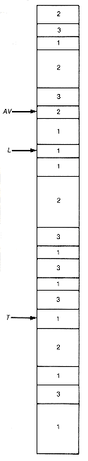
Figure 13.1 A Heap Containing the Available Space List (AV), a List (L), and a Binary Tree (T) and Nodes Labeled 1, 2, or 3 to Show Status
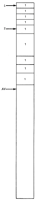
Figure 13.2 The Heap of Example 13.4 (Figure13.1) after Compaction
13.3.1 Two-Way Circular Lists
13.3.2 The Buddy System
 lg n
lg n . If a[k] is not null, a node is deleted from its list to satisfy the request. Otherwise, the next nonnull list is found. Its nodes will be of length 2r, where r > k. A node is deleted from that list and split into two nodes, each of length 2r-1. That node created by the split with the greater address is placed on the appropriate list, while the other is used to satisfy the request if r - 1 = k. Otherwise it is split and processed in the same way. Eventually a node of length k will be generated to satisfy the request.
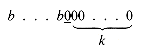
(a) After a Sequence of Requests Is Made for Nodes of Size 8, 16, 4, 6
(b) After the Node of Length 16 Is Returned
Figure 13.3 Sequence of Memory Configurations for Example 13.6
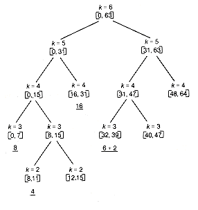
Figure 13.4 Binary Tree Reflecting the Memory Configuration for Example 13.6 Just before Return of Node of Length 16
13.3.3 Indexing Methods
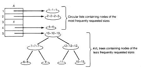
Figure 13.5 An Indexing Array Containing Pointers to Circular Lists and an AVL Tree Storing Circular Lists
13.4: Shared Storage

Figure 13.6 A Shared Sublist
13.5: Storage Reclamation Techniques
13.5.1 Garbage Collection
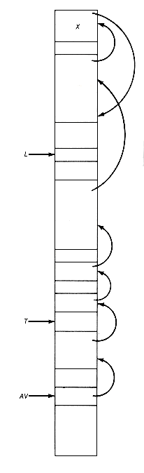
Figure 13.7 Heap from Example 13.4 after Garbage Collection
13.5.2 The Reference Counter Method

(a) Initial List Structures with Reference Counts

(b) Final List Structures with Reference Counts
Figure 13.8 List-structures of Figure 13.6 with Associated Reference Counts

Figure 13.9 A Lost Loop
13.5.3 Overview of Storage Reclamation
13.6: Stackless Traversals
preorder(pt)
/* Preorder traverses the binary tree. */
binarytreepointer *pt;
{binarytreepointer null,p,lptr,rptr;
binarytreepointer setnull(),left(),right(),nextsubtree();
stack s;
null = setnull();
p = *pt;
setstack(&s);
while(p != null)
{process(pt,p);
lptr = left(p);
if(lptr != null)
{push(p,&s);
p = lptr;
}
else
{rptr = right(p);
if(rptr != null)
{push(p,&s);
p = rptr;
}
else
p = nextsubtree(&s,&p);
}
}
}
Figure 13.10 A Binary Tree T
13.6.1 Threaded Trees
Routine Task
--------------------------------------------------------------------
setnull( ) determined by the implementation (array or pointer
variables)
setstack(&s) sets s to null
push(p,&s) sets s to p
left(p) returns a copy of leftptr.p if it is not a thread, and a
null value otherwise
right(p) similar to left(p)
nextsubtree(&s,&p) set s to p
while (rightptr.s is a thread),
set s to rightptr.s
return a copy of rightptr.s
13.6.2 Link Inversion

Figure 13.11 A Threaded Implementation of the Binary Tree T

Figure 13.12 A Link-inverted Binary Tree T
Routine Task
-----------------------------------------------------------------------------
setnull( ) determined by the implementation
setstack(&s) set s to null
push(p,&s) if leftptr.p is not null, then
set leftptr.p to s and s to p
else
set tag(p) to 1, set rightptr.p to s and s to p
left(p) returns a copy of leftptr.p
right(p) returns a copy of rightptr.p
nextsubtree(&s,&p) set found to false
while((not found) and (s not null))
if tag(s) = 1, then
set pred to s
set tag(s) to 0, s to rightptr.s,
rightptr.pred to p, and p to pred
else
set pred to leftptr.s and leftptr.s to p
if rightptr.s null, then
set found to true, tag(s) to 1, return
rightptr.s, and set rightptr.s to
pred
else
set p to s, set s to pred
if s = null, then
return null.

Figure 13.13 New State before Subtree Pointed to by P Is Traversed in Binary Tree T
13.6.3 Robson Traversal
Figure 13.14 Robson Traversal Configuration of the Binary Tree T

Figure 13.15 Robson Traversal before P Is Processed in the Binary Tree T
Routine Task
-----------------------------------------------------------------------------
setnull( ) determined by the implementation
setstack(&s) sets top, stack, and s to null
push(p,&s) if leftptr.p is not null then
set leftptr.p to s and s to p
else
set rightptr.p to s and s to p
left(p) returns a copy of leftptr.p
right(p) returns a copy of rightptr.p
nextsubtree(&s, &p) set avail to p
set found to false
while((not found) and (s not null))
if top = s, then
save stack in hold, pop the stack by setting
top to rightptr.stack, stack to leftptr.
stack, and leftptr.hold and
rightptr.hold to null. Save leftptr.s in
pred, restore leftptr.s by setting it to
rightptr.s, restore rightptr.s by setting it
to p, set p to s, and s to pred
else
if leftptr.s = null, then
save rightptr.s in pred, restore
rightptr.s by setting it to p, set p to s,
and s to pred
else
if rightptr.s null, then
push an entry for s onto the stack by
setting leftptr.avail to stack,
rightptr.avail to top, stack to
avail, and top to s. Return the value
of rightptr.s, set rightptr.s to p,
and set found to true
else
save leftptr.s in pred, restore
leftptr.s by setting it to p, set p to s,
and s to pred.
if s = null, then
return null.
13.7: Pitfalls: Garbage Generation and Dangling References
 leftptr is now on the list of available space. Rleftptr is called a dangling reference because it points to a node that is on the list of available space. When process is invoked in statement (5), it is possible that it invokes malloc, so storage is allocated to s. Then we have the situation shown in Figure 13.16(f).
(a) Initial Situation

(b) Result of Statement (1)

(c) Result of Statement (2)

(d) Result of Statement (3)

(e) Result of Statement (4)

(f) Result of Statement (5)

(g) Result of Statement (6)
Figure 13.16 Simulation of the Disaster Segment
13.8: Conclusion
Exercises
 10. 50. If the [i,j] entry of the array is 1, then node j is a successor of node i; if the [i,j] entry is 0, then node j is not a successor of node i.
Suggested Assignments