Binary trees can be used as the basis for encoding text and for the creation of Huffman codes. Binary search trees can also be used to generate more quickly codes of comparable efficiency.
The application of "simple" and balanced binary search trees for record storage and retrieval by key was demonstrated in Chapter 9. As shown there, "simple" binary search trees provide excellent average search times with random input when keys are accessed equally often. Also, AVL trees guarantee excellent worst-case search time. We shall see in this chapter that optimal binary search trees are useful when the keys have known, even unequal, frequencies, and when the trees, once grown, remain unchanged. Words in English text occur with known and unequal frequencies. An optimal binary search tree could be applied, for example, as a dictionary storing the 500 most frequently used English words, along with their definitions and their common misspellings. A search of the tree would then yield the definitions and misspellings. Once built, this tree would remain unchanged.
This chapter shows that the problems of finding Huffman codes and of finding optimal or nearly optimal binary search trees are related. The solutions illustrate the use of trees, heaps, and list-structures in the construction of good algorithms. The chapter also introduces the "greedy" heuristic. This method leads to an optimal solution for finding Huffman codes and to a nearly optimal solution for finding binary search trees. In both cases, the proper selection of data structures plays a significant role.
An important measure associated with binary trees is the weighted path length. This measure underlies the entire development in this chapter. Suppose a numeric weight is assigned to each node of a binary tree T. The meaning of these weights is dependent on the intended application. When the application of the binary tree is to text compression or text encoding, only the weights assigned to terminal nodes have meaning. Each terminal node corresponds to a different character that can appear in the text. The weight assigned to the node represents the relative number of occurrences of the character in the text. When the binary tree is used for record storage, each node stores a record with a particular key. The weight assigned to a node represents the frequency of search requests for the key corresponding to the node. These weights must be estimated or determined empirically for each specific application.
The weighted path length of a node in T is the product of its depth and its assigned weight. The weighted path length of T, W(T), is the sum of the weighted path lengths of all nodes of T. As an example, consider the binary tree in Figure 12.1(a), with assigned weights indicated for each node. Its weighted path length is
or 302. This was calculated directly from the definition of the weighted path length.
Another way to determine the weighted path length is to determine first the value of each node of the tree. The value of a node is the sum of the assigned weights of all nodes in the subtree with that node as root. Thus the root of a tree is assigned a value that is the sum of all the weights of the tree. The example would have values assigned to each node as indicated in Figure 12.1(b). The weighted path length of the tree is then calculated by adding up the values of the nodes.Thus, from Figure 12.1(b), the weighted path length is
It is easy to see that adding the node values must always yield the weighted path length, since the weight of any node is counted once for every subtree in which it appears. For example, the weight 31 is counted in the value attached to each node from the node to which it is assigned to the root. This is a total of four nodes, exactly the number of times that the node's weight should count in the weighted path length.
The weighted path length can be viewed in still another way. It is given by the value of the root plus the weighted path length of the two subtrees of the root node. For the example shown in Figure 12.1(b), this is given by 100 + 152 + 50, where 100 is the root's value and 152 and 50 are the respective weighted path lengths of the left and right subtrees. Thus there are three ways in which the weighted path length of a binary tree can be calculated.
With this background, let us turn to Huffman coding itself. First we will look at how information may be coded based on a binary tree and how it is coded in computers. Consider a binary tree with n terminal nodes. Assign a zero to every left successor branch and a one to every right successor branch of the tree. Encode each terminal node with the sequence of 0's and l's encountered when following the path from the root to the terminal node. Since this path is unique, the sequence or code assigned to each node must be unique. For example, in binary tree T1 (shown in Figure 12.2) the twenty-six letters of the alphabet and the space character designated by
The code assigned to the letter S in T1 is the sequence 00011 of length 5, one less than the depth of the encoded node to which S is assigned. In this way, a code is automatically generated for the twenty-seven characters associated with the terminal nodes of T1. Any string of these characters can then be encoded into a string of 0's and 1's. This string is simply the sequence of the combined sequences of 0's and l's that constitute the codes for each of the characters in the string. For instance, the string of six characters "A
of length 18. Again, because each path is unique, given any two code words, one can never be an extension of another. Consequently, no other sequence of code words will yield exactly this sequence of eighteen 0's and 1's, and any sequence starting with these eighteen 0's and 1's must start with A
The tree T1 generates a variable-length code, since it does not assign the same length sequences of 0's and 1's to each character. A fixed-length code assigns equal-length strings of 0's and 1's to each character. A fixed-length code would be generated by a tree if each terminal node of the tree had the same depth.
Since elements of computer memory actually store only sequences of 0's and 1's (by design), character information must be encoded. One way to encode the character set of a computer is by means of a standard fixed-length code, which uses six 0's and 1's per character.
The character set of a computer is the alphabet of characters that it can accept. For example, not all computers accept braces (that is, {}). Two important standard character sets are ASCII (American Standard Code for Information Interchange) and EBCDIC (Extended Binary Coded Decimal Interchange Codes). Both use fixed-length codes. ASCII uses a seven-bit code and EBCDIC uses eight bits. An n-bit fixed-length code can distinguish 2n characters, and a sequence of l characters would then be represented by a sequence of l X n 0's and 1's. Variable-length codes are not constrained to using the same number of 0's and l's for each character.
Using a variable-length code, a text in which the characters occur with different frequencies can be compressed. Shorter-length sequences would be assigned to characters used more frequently, and longer-length sequences to characters used less frequently. This is the idea behind the Morse code. Morse, in fact, estimated the relative frequencies of characters by looking at the frequency with which printer's boxes containing the different characters of the alphabet needed to be refilled.
The use of fixed-length codes makes it easy to decode a sequence of 0's and 1's to recover the original sequence of characters or text. It is not so easy for variable-length codes. A variable-length code must be chosen with care, if it is to allow proper decoding and avoid ambiguity. One way to achieve such a code is to use the scheme outlined for Figure 12.2, which associates a code to each binary tree. Decoding the code generated by a given binary tree would then proceed as follows:
1. Start at the root of a binary tree that is identical to the one used for encoding the original text.
2. Follow the branches according to the dictates of the sequence of 0's and l's to be decoded--go left for a 0 and right for a 1.
3. When a terminal node is reached, the sequence of 0's and 1's that led to it is decoded as the character associated with that terminal node.
4. Start again at the root to decode the remainder of the sequence in the same way.
The relative frequency with which each of twenty-six characters of the alphabet and the blank space between words occur in English text is as follows:
These relative frequencies are used to assign weights to the nodes of a tree such as T1. Each internal node is assigned weight 0, and each terminal node is assigned the relative frequency of the character associated with it. Thus, node S of T1 is assigned weight 51. The average amount of compression is measured by the weighted path length of the tree. In this way, the amount of compression achieved with different codes can be compared, since each tree has associated with it a unique code. The average length of the assigned codes is obtained by subtracting 1 from the weighted path length when the weights are normalized to sum to 1. Weights are normalized by dividing each weight by the sum of all the weights. The designer of a compression scheme can make this calculation directly or write a program for this purpose.
The weighted path length of T1 can be improved. Take the subtree with root at depth 5, and I and S as its successors, and interchange it with T to obtain binary tree T2 (shown in Figure 12.3). The weights of I and S, 57 and 51, will now each contribute one less time to the weighted path length of T2 than to T1, while T, with weight 80, will contribute one more time to the weighted path length of T2 than to T1. The result is that the weighted path length of T2 will be (57 + 51) - 80 less than that of T1.
The programmer's goal should be to find a binary tree, called the optimal binary tree, which has minimum weighted path length when the characters of the alphabet are stored at its n terminal nodes. Incidentally, the references here are to characters associated with the terminal nodes, but more generally they can be words or messages. A straightforward algorithm for finding this optimal binary tree is to generate each binary tree with n terminal nodes, associate the alphabetic characters with these n nodes, and calculate the weighted path length of the tree. A tree that yields the minimal weighted path length is optimal. Unfortunately, this algorithm is feasible only for small n. If n = 13, there are more than 1012 such trees, and the number of trees increases by a factor of almost 4 each time n increases by 1. We have to find a better way.
An optimal binary tree generates what is called a Huffman code. Fortunately, the searching just described is not needed to find it; it can be constructed as follows.
1. Start with a collection of n trees, each with just a root. Assign an alphabetic character to each of these nodes. The weight of each node is the weight associated with its alphabetic character. The value of each of these root nodes is equivalent to its weight. (Value in this case equals the weight of the root itself, since these trees have no other nodes.)
2. Find the two trees with smallest values. Combine them as the successors of a tree whose root has a value that is the sum of their values. Remove the two combined trees and add the new tree obtained to the current collection of trees. Repeat the second step n - 2 times to obtain exactly one tree. This will be the optimal tree and will give the assignments of characters to terminal nodes.
When this algorithm is applied to the twenty-seven characters with their weights reflecting their frequency of occurrence in English, the first combination made is J with Q, since each has weight 1. The resultant tree has value 2. Next X and Z, also each of weight 1, are combined, yielding another tree with value 2. These two trees are combined, yielding a tree with value 4. The current collection now consists of twenty-four trees. The next combination involves weights 4 and 5 and yields value 9. Following this procedure, a final optimal tree that might result from the construction is shown in Figure 12.4. Other optimal trees could have been constructed, but all would have the same weighted path length of 5,124. This means that the average length (number) of 0's and 1's needed per character will be 4.124. The value 4.124 is obtained by normalizing the weighted path length (dividing it by the sum of the weights) and subtracting one. Thus 5124/1000 - 1 = 4.124. This saves almost 20 percent over a fixed-length code of length 5 (the shortest fixed-length code that can distinguish twenty-seven characters).
This construction procedure is the Huffman algorithm. A proof is given later showing that it does, in fact, produce an optimal binary tree. Notice that a cumulative total weight can be kept as the algorithm is carried out. To do this, start with the variable weight set at the sum of all the weights of the alphabetic characters. Every time two trees are combined, add the value of the resultant tree to weight. When the algorithm terminates, after making (n - 1) combinations, weight will contain the weighted path length of the optimal binary tree constructed.
The algorithm chooses the combination of current trees that yields a minimal value for the combined trees. It is in this sense that it is a "greedy" algorithm. It doesn't consider future ramifications of the current choice of subtrees to combine but takes the current two "best" subtrees. In this instance, best means "of smallest value." The algorithm makes a "local" best or greedy decision. It is an example of the greedy method of algorithm design, which involves making choices on the basis of the immediate best alternative. This may lead to later choices being constrained to such poor alternatives as to lead to an overall suboptimal result. Being less greedy now may lead to better choices later, which in turn may yield better overall results. Hence it is not obvious that taking the best possible next combination, as done here, must lead to an optimal tree.
The greedy method does not yield optimal solutions in all situations. A traveler who applied the greedy method to selecting a route might always choose the next road because it is the shortest of all the current possibilities. This method will clearly not always yield the shortest overall route. When making change in U.S. currency using our system of 1-, 5-, 10-, 25-, and 50-cent pieces and dollar bills, we normally use a greedy algorithm. For instance, to give $3.70 change most people would give three $1 bills, one 50-cent piece, and two dimes (not seven 50-cent pieces, one dime, and two nickels). The algorithm is greedy because it always takes as many pieces of currency of the next largest value as possible. This always minimizes the total number of pieces of currency used to make change in our system. If a system had 1-, 5-, and 11-cent pieces and dollar bills, then making change "greedily" to give $3.70 would require three $1 bills, six 11-cent pieces, and four pennies. Fewer pieces of currency result from using three dollar bills, five 11-cent pieces, and three nickels, Fortunately, the greedy method does yield optimal binary trees.
Let us now consider how the binary tree constructed by the Huffman algorithm should be stored in memory. To this end we consider an example that shows that even though the weighted path length is as small as possible for a given set of weights, the depth of the tree can still be great.
Example 12.1
Suppose that the first n Fibonacci* numbers are assigned as weights to characters of an alphabet represented as terminal nodes in a tree. The task is to generate a Huffman code.
*The Fibonacci sequence is the sequence of integers F0, F1, F2, . . . that starts with F0 = 0 and F1 = 1, with each succeeding integer found by adding its two predecessors. Thus the sequence is 0, 1, 1, 2, 3, 5, 8, 13, 21, 34, 55, . . . , Fn-1, . . . , where F0 = 0, F1 = 1, Fn+2 = Fn+1 + Fn, n
The Huffman algorithm would construct the tree shown in Figure 12.5. This tree has depth n. Hence the Huffman algorithm may generate trees whose depth is O(n). If a sequential representation were used for such trees, considerable storage would be wasted. For large n, the storage would not even be available. A good alternative is a linked representation of the tree.
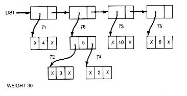
In this section the Huffman algorithm is implemented so that the Huffman tree and its weighted path length are generated. For a list of n records, a linked representation of the tree is illustrated in Figure 12.6(a) for n = 5 and weights 4, 3, 10, 2, 6.
The X's in the figure represent null pointers. The information field of each list record contains a pointer to a record representing the root of a binary tree. The records of the tree might be stored using pointer variables or in arrays. The records have leftptr, info, and rightptr fields. The info field contains the value assigned to the record's subtree by the Huffman algorithm. Thus each list record represents a tree. Weight is a variable initially set to the sum of the n weights and incremented by the value attached to each combined tree.
The implementation could proceed by traversing the list to find the trees with the two smallest values. These trees must be combined as dictated by step 2 of the algorithm into a new tree whose value is the sum of their values. The two trees that were combined must be deleted from the list, and the new tree added to the list. The result of these operations is shown in Figure 12.6(b) after one combination has taken place.
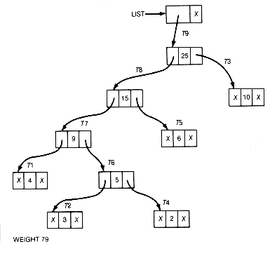
Every time step 2 is repeated, two trees are combined and the length of the list decreases by 1. The final list would contain one record; its information field would point to the root of the generated Huffman tree. Weight would contain its weighted path length. For this example, the resultant list would be as shown in Figure 12.6(c).
The list traversal required to find the two smallest value trees results in a worst-case time proportional to the length of the list for each traversal. Since the tree must be traversed n - 1 times, the worst-case time is O(n2). We can do better.
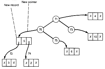
To improve the implementation, the two smallest values whose trees are to be combined must be found quickly without traversing the entire list. Recall that a heap, in this case a min heap, always has its smallest record at its root. Suppose the records of the binary tree are kept in a heap, or better, suppose the pointers are kept in the heap. Each pointer points to a corresponding record of the binary tree. The initial heap is shown in Figure 12.7.
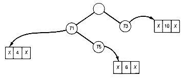
To find the two smallest values, simply remove the top heap pointer T4, reheap, and again remove the top pointer, T2. The records corresponding to the two smallest values can be combined. The new pointer to the combined record can then be placed at the top of the heap (which was left vacant), and the heap reheaped. Figure 12.7(b) shows the heap obtained by removing T4, reheaping, and removing T2. The two trees removed are combined, and reheaping is done to obtain the heap shown in Figure 12.7(c).
With this implementation the computer time consumed in finding the two smallest values, combining their corresponding records, and reheaping is O(lg n). Since the entire process is repeated (n - 1) times, the total time will be O(n lg n). It was the proper choice of data structure that made this improvement possible!
For those readers who would like a proof of the Huffman construction, the following is an interesting example of the use of mathematical induction applied to trees. It can easily be adopted to prove that a recursive program for the Huffman algorithm is correct.
Assume the weights are w1, w2, . . . , wn and are indexed so that w1
*See Exercise 5.
Given any tree with n terminal nodes, Tn, in which Figure 12.8(a) appears as a subtree, let T'n - 1 be the tree with n - 1 terminal nodes obtained from Tn by replacing this subtree by the terminal node shown in Figure 12.8(b). Then the weighted path length of Tn equals the weighted path length of T'n - 1 + (w1 + w2).
Given T'n-1, inversely, Tn can be obtained from it. Therefore, Tn must be optimal with respect to weights w1, w2 . . . , wn, if and only if T'n-1 is optimal with respect to weights (w1 + w2), w3, . . . , wn. This is because if only one tree were not optimal, it could be replaced by an optimal tree, thus improving the weighted path length of the corresponding version of the other.
By the induction hypothesis, the Huffman construction yields a tree, T'n-1, with n - 1 terminal nodes, that is optimal with respect to weights (w1 + w2), w3, . . . , wn. The corresponding tree, Tn, with n terminal nodes, is just the tree given by the Huffman construction for weights w1, w2 , . . . , wn . Since T'n-1 is optimal, so is Tn. This completes the proof.
So far we have been considering binary trees with nonzero weights assigned only to terminal nodes. Information (a character or message) has been associated only with their terminal nodes. We now consider extended binary search trees, which have keys stored at their internal nodes.
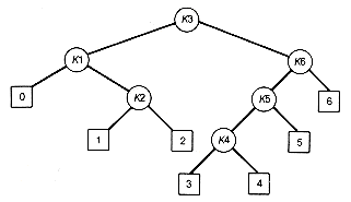
Suppose n keys, k1, k2, . . . , kn, are stored at the internal nodes of a binary search tree. It is assumed that the keys are given in sorted order, so that k1 < k2 < . . . < kn. An extended binary search tree is obtained from the binary search tree by adding successor nodes to each of its terminal nodes as indicated in Figure 12.9 by 's.
Although the programming goal in this chapter is to find optimal binary search trees, extended binary search trees are used along the way. In the extended tree, the 's represent terminal nodes, while the other nodes are internal nodes. These terminal nodes represent unsuccessful searches of the tree for key values. Such searches do not end successfully because the search key is not actually stored in the tree. They actually terminate when a null subtree pointer is encountered along the search path.
In general, the terminal node in the extended tree that is the left successor of k1 can be interpreted as representing all key values that are not stored and are less than k1. Similarly, the terminal node in the extended tree that is the right successor of kn represents all key values not stored in the tree that are greater than kn. The terminal node that is accessed between ki and ki+1 in an inorder traversal represents all key values not stored that lie between ki and ki+1. For example, in the extended tree in Figure 12.9(b), if the possible key values are 0,1, 2, 3, . . . ,100, then the terminal node labeled 0 represents the missing key values 0,1, and 2 if k1 is 3. The terminal node labeled 3 represents the key values between k3 and k4. If k3 is 17 and k4 is 21, then the terminal node labeled 3 represents the missing key values 18,19, and 20. If k6 is 90, then terminal node 6 represents the missing key values 91 through 100.
Assuming that the relative frequency with which each key value is accessed is known, weights can be assigned to each node of the extended tree. The weights represent the relative frequencies of searches terminating at each node. The weighted path length of the extended tree is then a natural measure for the average time to search the binary search tree for a key.
Example 12.2
Find the extended binary search tree that has the minimal weighted path length. The optimal binary search tree is obtained from this tree simply by omitting the extended nodes.
Before dealing with this problem, we compare it to the Huffman coding problem that has already been solved. When the weights attached to the internal nodes of the extended binary search tree are zero, this problem is similar to the Huffman coding problem. The difference is that the task now is to find the binary search tree with minimal weighted path length, whereas the Huffman algorithm finds the binary tree with minimal weighted path length. Since the binary search trees are only a subset of all binary trees, the Huffman tree will yield a value of the minimal weighted path length that is never larger than that of the optimal binary search tree. The Huffman algorithm will not solve the current problem unless, by chance, the tree that it constructs is a binary search tree or can be converted to one with no increase in the weighted path length. An algorithm, the Hu-Tucker algorithm, has been developed for this special case, and requires, as does the Huffman algorithm, time O(n lg n) and O(n) storage. Initially, its time was thought to be O(n2), but Knuth showed how to reduce this time by selecting the appropriate data structure. We now proceed to the general case in which the weights of the internal nodes need not be zero.
An obvious way to find an optimal binary search tree is to generate each possible binary search tree for the keys, calculate its weighted path length, and keep that tree with the smallest weighted path length. This search through all possible solutions is not feasible except for small n, since the number of such trees grows exponentially with n. A feasible alternative would be a recursive algorithm based on the structure inherent in optimal binary search trees. Such an algorithm can be developed in a way similar to that used for the construction of Fibonacci trees in Chapter 7.
How do we decompose the optimal search tree problem in Example 12.2 into components with the same structure? Consider the characteristics of any optimal tree. Of course, it has a root and two subtrees. A moment's reflection should convince you that both subtrees must themselves be optimal binary search trees with respect to their keys and weights. First, any subtree of any binary search tree must be a binary search tree. Second, the subtrees must also be optimal. Otherwise, they could be replaced by optimal subtrees with smaller weighted path lengths, which would imply that the original tree could not have been optimal.
Since there are n possible keys as candidates for the root of the optimal tree, the recursive solution must try them all. For each candidate key as root, all keys less than that key must appear in its left subtree, and all keys greater than it must appear in its right subtree. To state the recursive algorithm based on these observations requires some notation.
Denote the weights assigned to the n stored keys by
The optimal tree with root constrained to be kk and containing keys ki, . . . , kk, . . . , kj must then have obst(i,k-1) as its left subtree and obst(k+1,...,j) as its right subtree. Its weighted path length, w(i, j), is given by sw(i, j) + w(i, k - 1) + w(k + 1, j), where sw(i, j) is the sum of the weights
Finally the algorithm can be stated.
For each k(k) as root, k = 1, 2, . . . , n
find obst(1,k-1) and obst(k+1,n).
Find a k that minimizes [w(1, k - 1) + w(k + 1, n)] over k = 1, 2, . . . , n.
Obst(1,n) is given by the tree with root kk, obst(1,k-1) as its left subtree, and
obst(k+1,n) as its right subtree.
The weighted path length of obst(1,n) is w(1, n).
w(1, n) = sw(1, n) + w(1, k-1) + w(k+1, n).
The execution tree for obst(1,4) is given in Figure 12.10. Apparently this algorithm exhibits the same proliferation of recursive calls for identical component problems as did the algorithm for the Fibonacci tree construction in Chapter 7. These are summarized in Table 12.1. This inefficiency can be avoided by using a bottom-up construction, just as was done for Fibonacci trees. To do this requires a clear understanding of exactly which optimal subtrees must be retained for later reference.
All possible optimal subtrees are not required. Those that are needed consist of sequences of keys that are immediate successors of the smallest key in the
subtree, successors in the sorted order for the keys. The final solution tree contains all n keys. There will be two with n - 1 keys, three with n - 2 keys, four with n - 3 keys, and in general k + 1 with n - k keys, for k = 0, 1, 2, . . . , n. Consequently there are a total of (n + 1) X (n + 2)/2 optimal subtrees to be retained. Notice that to determine obst(i,j) requires knowing the optimal smaller subtrees involving weights:
The bottom-up approach generates all smallest required optimal subtrees first, then all next smallest, and so on until the final solution involving all the weights is found. Since the algorithm requires access to each subtree's weighted path length, these weighted path lengths must also be retained to avoid their recalculation. Finally, the root of each subtree must also be stored for reference.
This algorithm requires O(n3) execution time and O(n2) storage. Knuth, who developed this solution, noticed an important fact that reduces the execution time to O(n2). He was able to show that the minimization need not be over all k from 1 to n. Instead, the minimization may be taken only over all k between r(i,j - 1) and r(i + 1,j), where r(i,j) denotes the root of obst(i,j). See Knuth [1973b].
Intuitively, this is plausible because obst(i,j-1) is the optimal binary search tree containing keys ki, . . . , kr(i,j-1), . . . , kj-1. Thus taking kr(i,j-1) as its root gives the tree just the "balance" it needs to be optimal, distributing keys to its left and right subtrees in the optimal way. Obst(i,j) includes kj as well. If its root is also kr(i,j-1), then kj will appear in the right subtree of this optimal tree adding more weight to its right subtree. Think of the optimal tree as "balanced." Its root should not be a predecessor of kr(i,j-1), since this would cause even more weight to appear in its right subtree. Reasoning this way, it is not unreasonable to expect the root of obst(i,j) to be kr(i,j-1) or one of its successors. Thus looking only at k where r(i, j - 1)
The bottom-up algorithm, incorporating the new minimization limits, may now be written.
1. For i from 0 to n
a. Set w(i + 1, i) to 0 and sw(i + 1, i) to
b. For j from i + 1 to n
Set sw(i + 1, j) to sw(i + 1, j - 1) +
2. For j from 1 to n
a. Set w(j, j) to sw(j, j) and r(j, j) to j.
(This initializes all obst's containing 0 keys and 1 key.)
3. For l from 2 to n
a. For j from l to n,
i. set i to j - l + 1;
ii set w(i, j) to sw(i, j) + minimum[w(i, k - 1) + w(k + 1,j)], the minimum to be over k satisfying r(i, j - 1)
Actually, the w(i,j)'s will differ from the weighted path length of obst(i,j) by the sum of
Arrays for w, ws, and r seem to be a natural choice for implementing this algorithm and provide rapid access to the information required for the processing involved.
Example 12.3
Find the optimal binary search tree for n = 6 and weights
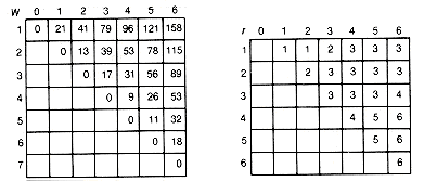
Figure 12.11(a) shows the arrays as they would appear after the initialization, and 12.11(b) gives their final disposition. The actual optimal tree is shown in Figure 12.12. It has a weighted path length of 188.
Since this algorithm requires O(n2 ) time and O(n2) storage, as n increases, it will run out of storage even before it runs out of time. The storage needed can be reduced by almost half, at the expense of a slight increase in time, by implementing the two-dimensional arrays as one-dimensional arrays using the technique of Chapter 2. Using one-dimensional arrays may enable problems to be solved that otherwise will abort because of insufficient storage. In any case, the algorithm is feasible only for moderate values of n.
In order to understand exactly how the algorithm creates the optimal tree, you should simulate the algorithm to reproduce the arrays of Figure 12.11.
To date, no one knows how to construct the optimal binary search tree using less time or storage in the general case of nonzero
One such algorithm produces greedy binary search trees. These trees are constructed by an algorithm using the greedy method. Unlike the Huffman algorithm, which is also based on the greedy method, they are not guaranteed to be optimal, but they are guaranteed to be nearly optimal. Other distinct, nearly optimal, tree constructions are found in Mehlhorn [1975, 1977] and in Horibe and Nemetz [1979]. A comparison of all these and other algorithms for the generation of nearly optimal binary search trees appears in Korsh [1982]. The proof that the following greedy method yields nearly optimal trees is in Korsh [1981].
In constructing a nearly optimal binary search tree by the greedy method, the programmer must ensure that the solution is a binary search tree. Looking at the optimal tree (Figure 12.12) found by the preceding section's algorithm will provide the idea behind the greedy tree construction. Think of the tree being generated by creating the subtrees shown in Figure 12.13, one after another, starting with the subtree with k4 at its root and ending with the final optimal tree. Each subtree has its value (the sum of its weights) associated with it.
Each subtree is formed by taking for its root a key that has not yet appeared and adjoining a left and right subtree. These subtrees may correspond to an extended node (with weight some
To start the development, we use the
Combining the corresponding key and terminal nodes yields the subtree shown in Figure 12.14(c). Its assigned value is the triple value 9. Delete that triple from the array, and replace it by a terminal node value of 9, as shown in Figure 12.14(d).
Now repeat this process. The next minimal value is 13, corresponding to the triple This gives the subtree shown in Figure 12.14(e). The condensed array is shown in Figure 12.14(f). Repeating the process finds the minimal triple whose value is 17. The corresponding subtree is Figure 12.14(g), and the new array is shown in Figure 12.14(h). Continuing in this fashion produces the arrays shown in Figure 12.14(i), (j), and (k).
The greedy tree thus constructed by always taking a minimal triple is shown in Figure 12.15. Its weighted path length can be found by keeping an accumulated sum, as in the Huffman algorithm. In this case the greedy algorithm actually yields the optimal tree.
Just as in the Huffman tree construction, if we are not careful we will end up with an O(n2) time implementation. Instead, we can use a heap similar to that for the Huffman construction to obtain an O(n 1g n) time requirement and O(n) storage. However, we can do even better.
The preceding method leads to a sequence of n - 1 combined triples with values v1, v2, . . . , vn-1. In this sequence v1
We start with a list-structure illustrated in Figure 12.16. Each record represents a potential triple to be combined in the construction of a greedy tree. Traverse the list starting at the left and search for a locally minimal triple -- that is, a triple whose value does not exceed the value of its successor triple. No triple to the left of this locally minimal triple can be combined before it in any greedy tree construction. In addition, any future combining of locally minimal triples to its right cannot cause the resultant tree to fail to be greedy. In other words, combining the minimal triple always allows a greedy tree to be constructed with the combined minimal triple as a subtree. Combine the locally minimal triple (say it is the ith), and obtain the new list-structure shown in Figure 12.16(b).
Here
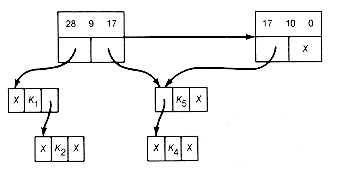
Applying this improved algorithm to Example 12.3, the starting list-structure is as shown in Figure 12.16(c). The first locally minimal triple found is 6 3 4. The list-structure resulting from combining it is shown in Figure 12.16(d). Starting again at the first record, 4 2 3 is the next minimal triple, yielding the list shown in Figure 12.16(e). Starting again, the first record here is found to be the locally minimal triple to obtain the list shown in Figure 12.16(f).
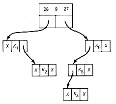
Starting again at the next first record, 9 0 8, the next locally minimal triple, gives the list shown in Figure 12.16(g). Once again, we start at the first record. The next locally minimal triple is 17 10 0. Combining it results in Figure 12.16(h). Finally the triple 28 9 27 is combined to obtain the result shown in Figure 12.16(i).
We have constructed the same tree as before (in Figures 12.14 and 12.15). Again, this need not always occur. However, even when it does, as here, the order in which the subtrees were formed need not be the same. We generated subtrees with values 13, 9, 28, 17, 27, and finally 64, rather than in order from the smallest to largest as in the other method. Both trees in this example have the same weighted path length of 188.
This implementation takes time and storage only O(n)! This was made possible by the new method, coupled with the proper choice of data structure.
Consider the twenty-seven characters with relative frequencies given in Section 12.3 as weights. Order them as
Binary trees are useful data structures for encoding and decoding information. The Huffman algorithm generates optimal binary trees for this purpose and can do so efficiently. Binary search trees are useful data structures for storing information that is to be searched; they also produce good codes.
Greedy binary search trees, which are nearly optimal, can be generated very efficiently. The greedy method of algorithm design does not yield optimal solutions but may still yield very good solutions. Again it was demonstrated that careful selection of data structures can significantly change the time requirements of an algorithm.
1. a. Using its definition, calculate the weighted path length of the following tree. The weight of a node appears at the node.
b. Calculate the weighted path length of the tree using the other method of assigning a "value" to each node and adding up all the "values."
c. Calculate the weighted path length of the same tree by adding the sum of all its weights to the weighted path length of its left subtree plus the weighted path of its right subtree.
2. Write a process function to turn a postorder traversal into a function for determining the weighted path length of a binary tree T based on the method of Exercise 1(b).
3. Determine the Huffman code (tree) for weights 1, 2, 3, 4, 5.
4. Determine the weighted path length for your solution to Exercise 3.
5. The Huffman tree for n weights will always have (n - 1) internal nodes and n terminal nodes. This is because it is a full binary tree. That is, every internal node has exactly 0 or exactly two successors. Prove, by induction on the total number of nodes of a full binary tree, that this is true.
6. Write a nonrecursive function, huffman, with parameters n, weights, tree, and code. Weights is an array containing n weights, code is an array returned containing the n codes (sequences of 0's and 1's) assigned to each weight by the Huffman code, and tree points to the root of the corresponding Huffman tree upon return. Your function should take O(n 1g n) time.
7. Write a recursive version of the function of Exercise 6.
8. Simulate the proof (by induction on n) that the Huffman tree yields a binary tree with minimal weighted path length for n weights for Exercise 3.
9. Write a function decode with parameters n, alpha, and tree. Alpha is a sequence of n 0's and 1's, and tree points to a Huffman tree for the twenty-seven characters of Section 12.3 (determined by their weights). Decode is to decode the sequence of n 0's and 1's into the corresponding characters. The sequence represents a coded version of a message composed of the characters.
10. Suppose you know the Huffman tree for the twenty-seven characters of Section 12.3 (determined by their weights). Write a function encode to encode a message composed of characters into the Huffman code. To do this you might consider using the following data structures:
a. The Huffman tree.
b. An array with twenty-seven records kept in sorted order by character, each record containing a character and its corresponding Huffman code.
c. A hash table of records, each record consisting of a character and its Huffman code; the key is the character.
Discuss the relative advantages and disadvantages for each of these in the function encode.
11. Write a function encode to encode a message in a Huffman code.
12. Let
13. The recursive approach of Section 12.4.1 is based on the idea that an optimal binary search tree must have an optimal left and an optimal right subtree. Can you use this idea to show that some of the trees you considered in Exercise 12 could have been ignored in searching for the optimal tree?
14. Simulate the bottom-up algorithm of Section 12.4.1 to reproduce the arrays of Figure12.11.
15. Why do we want to find nearly optimal binary search trees rather than optimal binary search trees for large numbers of keys?
16. Find the greedy binary search tree for the weights of Exercise 12 using the definition of a greedy tree. Determine the relative difference between its weighted path length and the optimal value.
17. Find the greedy binary search tree for the weights of Exercise 12 using the implementation of the greedy tree construction. Is its weighted path length the same as the greedy tree of Exercise 16?
18. Write a nonrecursive function greedy to implement the greedy tree construction of Section 12.5.3.
19. Give a recursive definition of a greedy binary search tree.
20. Write a recursive function greedy to implement the greedy tree construction of Section 12.5.3.
21. Another method of constructing a nearly optimal binary search tree is to select the key to be placed at the root to be a key that minimizes the difference between the weights of its left and right subtrees. Having obtained the root, apply this procedure recursively to construct its left and right subtrees. This is a top-down construction, as opposed to the greedy tree construction, which is bottom-up. What tree does it generate for the weights of Exercise 12 and for the example of Section 12.5.2?
22. Write a recursive function for the construction method of Exercise 21. How much time does your function require?
23. Can you find a way to implement the procedure of Exercise 21 in O(n) time, where n is the number of internal keys to be stored?
24. What will a greedy tree look like if the n
1. a. Write programs to find and output optimal greedy trees and their weighted path lengths.
b. Explain why the greedy tree implementation with the list structure is linear in time. (Hint: When the next locally minimal triple is to be found, only list-structure records not previously accessed will be considered, as well as two records that were previously accessed.)
2. a. Write a function to read a file composed of the twenty-six letters of the alphabet, plus the blank character, the comma, and the period; produce an output file that is the encoded version of the input file. The Huffman code is to be used, with weights based on the number of times each character appears in the input text.
b. This is the same as (a) except that the "words" of the input text are taken as the objects to be encoded, and their number of occurrences is the basis for the code. Use any reasonable definition of a word. For example, take commas, periods, blanks, and any sequence of other characters to be words.
Note: For both parts, use a function getnexttoken. In part (a) it must return the next character in the input or EOF, while in part (b) it must return the next word or EOF. Also, there must be a table in which the tokens (characters or words) are stored. This table must be searched for a token, inserted into, and its entries updated. Your function must treat the table with these operations as a data abstraction, so the solutions to both parts should look the same except that the definitions of certain functions should change from one solution to the other.
c. Run your program for part (b) with the table implemented as
i. a binary search tree
ii. a hash table using double hashing
iii. a table composed of two parts--an optimal binary search tree storing the 25 most frequently used English words (take the
d. Write a function to read a text file consisting of the twenty-six letters of the alphabet, plus the blank and period characters, and produce an output file consisting of the text in Huffman code. Use the heap implementation in generating the Huffman tree.
12.2: Weighted Path Length
(1
 3) + (2
  17) + (2
  10) + (3
  15) + (3
  0)
0) + (3
 20) + (4
  31) + (4
  4)
4)100 + 67 + 30 + 15 + 35 + 20 + 31 + 4 = 302
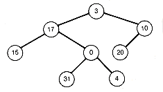
(a) Nodes Labeled with Assigned Weights
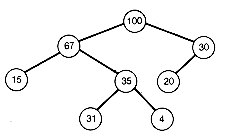
(b) Nodes Labeled with Values Derived by Adding Assigned Weights
Figure 12.1 Binary Tree T
12.3: Huffman Coding
 were assigned to the terminal nodes. Thus the code for the leftmost terminal node (N) in Figure 12.2 is the sequence 00000. Any character, word, or information associated with a terminal node is encoded with the unique code for that node.
 TREE" will be encoded
100101001100011111
 TREE.
TREE.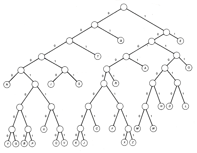
Figure 12.2 Binary Tree T1
 A B C D E F G H I J K L
186 64 13 22 32 103 21 15 47 57 1 5 32
M N O P Q R S T U V W X Y Z
20 57 63 15 1 48 51 80 23 8 18 1 16 1
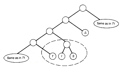
Figure 12.3 Binary Tree T2, Obtained by Interchanging Two Subtrees
12.3.1 The Huffman Algorithm
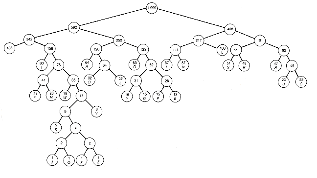
Figure 12.4 A Final Optimal Tree
12.3.2 Representation of Huffman Trees
 0.
0.
Figure 12.5 Tree Constructed by the Huffman Algorithm for Fibonacci Weights
12.3.3 Implementation

(a) List of Five Records Pointing to Five Initial Trees of the Huffman Algorithm
(b) List after Combining Two Trees with Smallest Values
(c) Final List and Huffman Tree after Repeated Combinings of Values
Figure 12.6 A Linked List Representing the Trees Constructed by the Huffman Algorithm

(a) Initial Heap
(b) Incomplete Heap
(c)Heap after Two Trees Are Combined and Reheaping Done
Figure 12.7 Heap of Pointers of the Huffman Tree
12.3.4 A Proof
 w2
w2  . . .
. . .  wn. You should convince yourself that an optimal binary tree must be a full binary tree.* An optimal tree can always be found, since the number of full binary trees with n terminal nodes is finite. It is clear that the Huffman construction yields optimal trees for n = 1 and 2. This is the basis for the induction, which will be on the number of weights or terminal nodes, n. The induction hypothesis is that the Huffman construction yields optimal trees for any n - 1 weights. We must show that as a result, it must generate optimal trees for n weights.
(a) Subtree

(b)Terminal Node after Combining Weights
Figure 12.8 Subtree Replacement
12.4: Optimal Binary Search Trees

(a) Binary Search Tree
(b) Extended Binary Search Tree
Figure 12.9 Extension of a Binary Search Tree
12.4.1 Finding Optimal Binary Search Trees
 's and the weights assigned to the terminal nodes by
  's. The weight assigned to ki is
  i for i = 1, 2, . . . , n, and that assigned to the external node labeled i is
  i for i = 0, 1, 2, . . . , n. Let obst(i,j) denote the optimal binary search tree containing keys ki, . . . , kj, and let w(i,j) denote its weighted path length. Obst(i,j) will involve weights
  i-1,
i-1,  i, . . . ,
  i,
i,  j.
j. i-1,
i-1,  i, . . . ,
  j,
j,  j. Sw(i, j) is the value assigned to the root of obst(i,j), the sum of its weights.
Table 12.1 Components Replicated by Recursive Calls
Replicated Component Occurrences
----------------------------------
(
 2,
2,  3,
3,  3,
3,  4,
4,  4) 2
4) 2 (
 0,
0,  1,
1,  1,
1,  2,
2,  2) 2
2) 2 (
 1,
1,  2,
2,  2,
2,  3,
3,  3) 2
3) 2 (
 0,
0,  1,
1,  1) 4
1) 4 (
 1,
1,  2,
2,  2) 5
2) 5 (
 2,
2,  3,
3,  3) 5
3) 5 (
 3,
3,  4,
4,  4) 4
4) 4 (
 0) 4
0) 4 (
 1) 3
1) 3 (
 2) 4
2) 4 (
 3) 3
3) 3 (
 4) 4
4) 4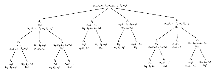
Figure 12.10 The Execution Tree for n = 4
(
 i-1) and (
 i,
i,  i+1, . . . ,
  j,
j,  j)
j)i.e., obst(i,i-1) and obst(i+1,j)
(
 i-1,
i-1,  i,
i,  i) and (
 i+1,
i+1,  i+2, . . . , Bj,
  j)
j)i.e., obst(i,i) and obst(i+2,j)
(
 i-1,
i-1,  i, . . . ,
  j-1,
j-1,  j-1) and (
 j)
j)i.e., obst(i,j-1) and obst(j+1,j)
 k should suffice. A symmetrical argument should make it equally reasonable that looking only at k, k
  r(i + 1, j) should suffice. The actual proof is complex and adds little insight, so it is omitted here.
 i
i j +
j +  j
j k
k  r(i + 1, j) and set r(i, j) to a value of k corresponding to the minimum.
 i-1,
i-1,  i, . . . ,
  j. This does not affect the final tree but means that to obtain the true weighted path length,
  0 +
0 +  1 + . . . +
  n must be added to w(1, n).
 1= 10,
  2= 3,
2= 3,  3= 9,
3= 9,  4= 2,
4= 2,  5= 0,
5= 0,  6= 10,
  0= 5,
0= 5,  1= 6,
1= 6,  2= 4,
2= 4,  3= 4,
3= 4,  4= 3,
4= 3,  5= 8,
5= 8,  6= 0.
6= 0. 
(a) Initial Array Values
(b) Final Array Values
Figure 12.11 Arrays Used to Implement the Bottom-up Recursive Algorithm for Finding Optimal Binary Search Trees
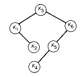
Figure 12.12 The Optimal Binary Search Tree Found by Means of the Bottom-up Recursive Algorithm
12.5: Nearly Optimal Binary Search Trees
 's and
  's. For this reason it is important to develop algorithms that produce good, but not necessarily optimal, solutions with less time and storage being required. Algorithms have been found that construct nearly optimal binary search trees. The weighted path lengths of such trees cannot differ by more than a constant factor from the optimal value.
12.5.1 Greedy Binary Search Trees
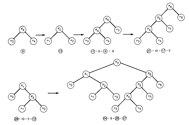
Figure 12.13 Trees Created from Subtrees (Circled Numbers Are the Trees' Values)
 i) or to an already produced subtree. The value of the subtree formed is given by the
  i of its key plus the value of its left and right subtrees. These subtrees must be selected in a constrained fashion, or the resultant tree will not be a binary search tree. These constraints will be delineated shortly, but for now, the main point is that the weighted path of the optimal tree is the sum of the values of each of the subtrees. The greedy trees are built by always selecting the next subtree to generate as the one with smallest value from among all those satisfying the constraints. This is exactly how the Huffman construction works, except there are no constraints on the choice of subtrees since the resultant tree need not be a binary search tree.
12.5.2 Greedy Construction
 's and
  's of Example 12.3 and array them as shown in Figure 12.14(a). In an inorder traversal of any binary search tree with the six keys, the weights assigned to the accessed nodes would occur in the order
  0
0  1
1  1
1  2
2  2
2  3, and so on. This sequence looks like triples, as shown in Figure12.14(b). A value can be associated with each triple by summing up its weights. Thus the triples just shown have values 21, 13, 17, 9, 11, and 18 respectively. A greedy tree is constructed by always finding an allowed triple with minimal value and generating its corresponding subtree next. The weighted path length of the resultant tree is the sum of the weights of the (n - 1) triples thus created. The greedy construction procedure is as follows. The allowable triples shown in the array have values 21, 13, 17, 9, 11, and 18. The triple with the lowest value (9) is
 2
4 3
3
6 4
 1
1  2
2  3
3  4
4  5
5  6
6 10 3 9 2 0 10
5 6 4 4 3 8 0
 0
0  1
1  2
2  3
3  4
4  5
5  6
6(a) Original Array of
 's and
  's from Example 12.3
(b) A Sequence of Triples

(c) Subtree with Value 9

(d) First Condensed Array

(e) Subtree with Value 13

(f) Second Condensed Array
Figure 12.14 Construction of Greedy Binary Search Tree

(g) Subtree with Value 17

(h) Third Condensed Array
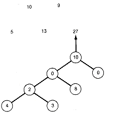
(i) Fourth Condensed Array
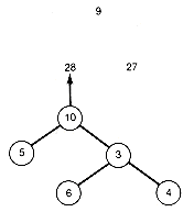
(j) Fifth Condensed Array

(k) Final Array
Figure 12.14
12.5.3 Implementation
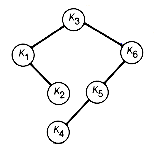
Figure 12.15 Greedy Binary Search Tree Constructed as Illustrated in Figure 12.14
 v2
v2  . . .
. . .  vn-1. That is, the triples are generated in order, from the smallest to the highest value. The improved algorithm, introduced now, also generates a sequence of n - 1 combined triples, but their values will not necessarily be the same as v1, . . . , v2, vn-1, nor will they necessarily be generated in order by size. The improved algorithm, however, will produce the greedy tree that would have been obtained had they been combined in order by size when it is unique. A unique tree exists when there is exactly one smallest triple at each step. In general, the resultant tree will be greedy, but it will not necessarily be the same greedy tree generated by v1, . . . , v2, vn-1, nor will it necessarily have the same weighted path length.
 'i-1 and
  'i were both set to the value of the combined triple
  'i-1 +
  i +
i +  'i, the ith record was deleted, and the pointers changed as shown. The left-to-right traversal is continued, starting now at the (i - 2)th record, combining as before for each locally minimal triple encountered. Details involving the ends of the list-structure can be handled by special checking or by introducing artificial records with large weights at the ends. This results in the construction of a greedy tree. This procedure is reminiscent of the evaluation of an infix expression of Chapter 4. That algorithm is greedy in the sense that we look for the highest local priority operator to evaluate first in a left-to-right scan, evaluate it, and continue from that point.
(a) Starting List Structure

(b) List Structure after Combining the ith Locally Minimal Triple

(c) Starting List Structure for the Weights of Example 12.3

(d) Result of Combining the Triple 6 3 4

(e) Result of Combining 4 2 3

(f) Result of Combining 5 10 13
(g) Result of Combining 9 0 8
(h) Result of Combining 17 10 0

(i) Result of Combining 28 9 27
Figure 12.16 Implementation of the Greedy Algorithm
12.5.4 Alphabetic Codes
 < A < B < C <

 < Z. Suppose we want to construct an extended binary search tree with these characters associated with the terminal nodes. We take the weights given there as the
  's of this problem and take the
  's to be zero. The extended binary tree will then generate what is called an alphabetic code. The optimal binary search tree will have weighted path length 5,200, and the greedy binary search tree will have weighted path length 5,307. Recall that the Huffman tree had weighted path length 5,124. Requiring use of a binary search tree rather than a binary tree results in an increase relative to 5,124 of only (5,200 - 5,124)/5,124 or 1.5 percent. The greedy construction yields an increase relative to 5,200 of (5,307 - 5,200)/5,200 or 2 percent.
12.6: Conclusion
Exercises

 0 = 10,
  1 = 6,
  2 = 8,
  3 = 4,
  4 = 2,
  1 = 2,
  2 = 5,
  3 = 7,
  4 = 6. Determine the optimal binary search tree by generating all possible binary search trees storing the four keys with weights 2, 5, 7, and 6, and calculating their weighted path lengths.
 's are zero and the n + 1
  's are given by the first n + 1 Fibonacci numbers? Give two answers--one when the greedy tree definition is used, and one when the O(n) implementation is used.
Suggested Assignments
 's to be zero) and a binary search storing any other words that occur in the input. The optimal binary search tree is to be built in advance of the input.


