After Section 31.1 introduces basic matrix concepts and notations, Section 31.2 presents Strassen's surprising algorithm for multiplying two n  n matrices in
  (nlg 7) = O(n2.81) time. Section 31.3 defines quasirings, rings, and fields, clarifying the assumptions required to make Strassen's algorithm work. It also contains an asymptotically fast algorithm for multiplying boolean matrices. Section 31.4 shows how to solve a set of linear equations using LUP decompositions. Then, Section 31.5 explores the close relationship between the problem of multiplying matrices and the problem of inverting a matrix. Finally, Section 31.6 discusses the important class of symmetric positive-definite matrices and shows how they can be used to find a least-squares solution to an overdetermined set of linear equations.
31.1 Properties of matrices
In this section, we review some basic concepts of matrix theory and some fundamental properties of matrices, focusing on those that will be needed in later sections.
Matrices and vectors
A matrix is a rectangular array of numbers. For example,

(31.1)
is a 2  3 matrix A = (aij), where for i = 1, 2 and j = 1, 2, 3, the element of the matrix in row i and column j is aij. We use uppercase letters to denote matrices and corresponding subscripted lowercase letters to denote their elements. The set of all m
  n matrices with real-valued entries is denoted Rm
 n. In general, the set of m
  n matrices with entries drawn from a set S is denoted Sm
 n.
n.
The transpose of a matrix A is the matrix AT obtained by exchanging the rows and columns of A. For the matrix A of equation (31.1),
A vector is a one-dimensional array of numbers. For example,
is a vector of size 3. We use lowercase letters to denote vectors, and we denote the ith element of a size-n vector x by xi, for i = 1, 2, . . . , n. We take the standard form of a vector to be as a column vector equivalent to an n
The unit vector ei is the vector whose ith element is 1 and all of whose other elements are 0. Usually, the size of a unit vector is clear from the context.
A zero matrix is a matrix whose every entry is 0. Such a matrix is often denoted 0, since the ambiguity between the number 0 and a matrix of 0's is usually easily resolved from context. If a matrix of 0's is intended, then the size of the matrix also needs to be derived from the context.
Square n
1. A diagonal matrix has aij = 0 whenever i
2 The n
When I appears without a subscript, its size can be derived from context. The ith column of an identity matrix is the unit vector ei.
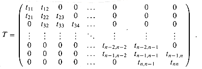
3. A tridiagonal matrix T is one for which tij = 0 if |i - j| > 1. Nonzero entries appear only on the main diagonal, immediately above the main diagonal (ti,i+1 for i = 1, 2, . . . , n - 1), or immediately below the main diagonal (ti+1,i for i = 1, 2, . . . , n - 1):
4. An upper-triangular matrix U is one for which uij = 0 if i > j. All entries below the diagonal are zero:
An upper-triangular matrix is unit upper-triangular if it has all 1's along the diagonal.
5. A lower-triangular matrix L is one for which lij = 0 if i < j. All entries above the diagonal are zero:
A lower-triangular matrix is unit lower-triangular if it has all 1's along the diagonal.
6. A permutation matrix P has exactly one 1 in each row or column, and 0's elsewhere. An example of a permutation matrix is
Such a matrix is called a permutation matrix because multiplying a vector x by a permutation matrix has the effect of permuting (rearranging) the elements of x.
7. A symmetric matrix A satisfies the condition A = AT. For example,
is a symmetric matrix.
The elements of a matrix or vector are numbers from a number system, such as the real numbers, the complex numbers, or integers modulo a prime. The number system defines how to add and multiply numbers. We can extend these definitions to encompass addition and multiplication of matrices.
We define matrix addition as follows. If A = (aij) and B = (bij) are m
for i = 1, 2, . . . , m and j = 1, 2, . . . , n. That is, matrix addition is performed componentwise. A zero matrix is the identity for matrix addition:
If
Given this definition, we can define matrix subtraction as the addition of the negative of a matrix: A - B = A + (-B).
We define matrix multiplication as follows. We start with two matrices A and B that are compatible in the sense that the number of columns of A equals the number of rows of B. (In general, an expression containing a matrix product AB is always assumed to imply that matrices A and B are compatible.) If A = (aij) is an m
for i = 1, 2, . . . , m and k = 1, 2, . . . , p. The procedure MATRIX-MULTIPLY in Section 26.1 implements matrix multiplication in the straightforward manner based on equation (31.3), assuming that the matrices are square: m = n = p. To multiply n
Matrices have many (but not all) of the algebraic properties typical of numbers. Identity matrices are identities for matrix multiplication:
for any m
Matrix multiplication is associative:
for compatible matrices A, B, and C. Matrix multiplication distributes over addition:
Multiplication of n
and
Matrix-vector products or vector-vector products are defined as if the vector were the equivalent n
is a number (actually a 1
Thus, the norm of x is its length in n-dimensional euclidean space.
We define the inverse of an n
Many nonzero n
If a matrix has an inverse, it is called invertible, or nonsingular. Matrix inverses, when they exist, are unique. (See Exercise 31.1-4.) If A and B are nonsingular n
The inverse operation commutes with the transpose operation:
The vectors x1, x2, . . . , xn are linearly dependent if there exist coefficients c1, c2, . . . , cn, not all of which are zero, such that c1x1 + c2x2 + . . . + cnxn = 0. For example, the vectors x1 = ( 1 2 3 )T, x2 = ( 2 6 4 )T, and x3 = ( 4 11 9 )T are linearly dependent, since 2x1 + 3x2 - 2x3 = 0. If vectors are not linearly dependent, they are linearly independent. For example, the columns of an identity matrix are linearly independent.
The column rank of a nonzero m
A square n
Theorem 31.1
A square matrix has full rank if and only if it is nonsingular.
An m
A null vector for a matrix A is a nonzero vector x such that Ax = 0. The following theorem, whose proof is left as Exercise 31.1-8, and its corollary relate the notions of column rank and singularity to null vectors.
Theorem 31.2
A matrix A has full column rank if and only if it does not have a null vector.
Corollary 31.3
A square matrix A is singular if and only if it has a null vector.
The ijth minor of an n
The term (-1)i+ j det(A[ij]) is known as the cofactor of the element aij.
The following theorems, whose proofs are omitted here, express fundamental properties of the determinant.
Theorem 31.4
The determinant of a square matrix A has the following properties:
Also, for any square matrices A and B, we have det (AB) = det(A) det(B).
Theorem 31.5
An n
Positive-definite matrices play an important role in many applications. An n
As we shall see, matrices that arise in applications are often positive-definite due to the following theorem.
Theorem 31.6
For any matrix A with full column rank, the matrix ATA is positive-definite.
Proof We must show that xT (ATA)x > 0 for any nonzero vector x. For any vector x,
Note that ||Ax||2 is just the sum of the squares of the elements of the vector Ax. Therefore, if ||Ax||2 = 0, every element of Ax is 0, which is to say Ax = 0. Since A has full column rank, Ax = 0 implies x = 0, by Theorem 31.2. Hence, AT A is positive-definite.
Other properties of positive-definite matrices will be explored in Section 31.6.
31.1-1
Prove that the product of two lower-triangular matrices is lower-triangular. Prove that the determinant of a (lower- or upper-) triangular matrix is equal to the product of its diagonal elements. Prove that the inverse of a lower-triangular matrix, if it exists, is lower-triangular.
31.1-2
Prove that if P is an n
31.1-3
Prove that (AB)T = BT AT and that AT A is always a symmetric matrix.
31.1-4
Prove that if B and C are inverses of A, then B = C.
31.1-5
Let A and B be n
31.1-6
Let A be a nonsingular n
31.1-7
Show that if A is a nonsingular symmetric matrix, then A-1 is symmetric. Show that if B is an arbitrary (compatible) matrix, then B ABT is symmetric.
31.1-8
Show that a matrix A has full column rank if and only if Ax = 0 implies x = 0. (Hint: Express the linear dependence of one column on the others as a matrix-vector equation.)
31.1-9
Prove that for any two compatible matrices A and B,
rank(AB)
where equality holds if either A or B is a nonsingular square matrix. (Hint: Use the alternate definition of the rank of a matrix.)
31.1-10
Given numbers x0, x1, . . . , xn-1, prove that the determinant of the Vandermonde matrix
is
(Hint: Multiply column i by -x0 and add it to column i + 1 for i = n - 1, n - 2, . . . , 1, and then use induction.)
This section presents Strassen's remarkable recursive algorithm for multiplying n
Strassen's algorithm can be viewed as an application of a familiar design technique: divide and conquer. Suppose we wish to compute the product C = AB, where each of A, B, and C are n
(Exercise 31.2-2 deals with the situation in which n is not an exact power of 2.) For convenience, the submatrices of A are labeled alphabetically from left to right, whereas those of B are labeled from top to bottom, in agreement with the way matrix multiplication is performed. Equation (31.9) corresponds to the four equations
Each of these four equations specifies two multiplications of n/2
Unfortunately, recurrence (31.14) has the solution T(n) =
Strassen discovered a different recursive approach that requires only 7 recursive multiplications of n/2
Strassen's method has four steps:
1. Divide the input matrices A and B into n/2
2. Using
3. Recursively compute the seven matrix products Pi = AiBi for i = 1, 2, . . . , 7.
4. Compute the desired submatrices r, s, t, u of the result matrix C by adding and/or subtracting various combinations of the Pi matrices, using only
Such a procedure satisfies the recurrence (31.15). All that we have to do now is fill in the missing details.
It is not clear exactly how Strassen discovered the submatrix products that are the key to making his algorithm work. Here, we reconstruct one plausible discovery method.
Let us guess that each matrix product Pi can be written in the form
where the coefficients
If we form all of our products in this manner, then we can use this method recursively without assuming commutativity of multiplication, since each product has all of the A submatrices on the left and all of the B submatrices on the right. This property is essential for the recursive application of this method, since matrix multiplication is not commutative.
For convenience, we shall use 4
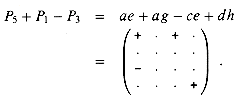
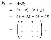
The last expression uses an abbreviated notation in which "+" represents +1, "
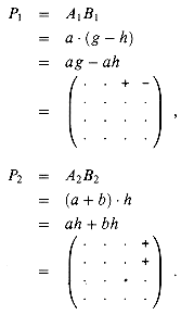
We begin our search for a faster matrix-multiplication algorithm by observing that the submatrix s can be computed as s = P1 + P2, where P1 and P2 are computed using one matrix multiplication each:
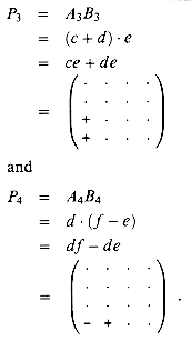
The matrix t can be computed in a similar manner as t = P3 + P4, where
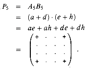
Let us define an essential term to be one of the eight terms appearing on the right-hand side of one of the equations (31.10)--(31.13). We have now used 4 products to compute the two submatrices s and t whose essential terms are ag, bh, ce, and df . Note that P1 computes the essential term ag, P2 computes the essential term bh, P3 computes the essential term ce, and P4 computes the essential term df. Thus, it remains for us to compute the remaining two submatrices r and u, whose essential terms are the diagonal terms ae, bf, cg, and dh, without using more than 3 additional products. We now try the innovation P5 in order to compute two essential terms at once:
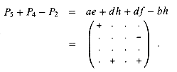
In addition to computing both of the essential terms ae and dh, P5 computes the inessential terms ah and de, which need to be cancelled somehow. We can use P4 and P2 to cancel them, but two other inessential terms then appear:
By adding an additional product
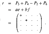
however, we obtain
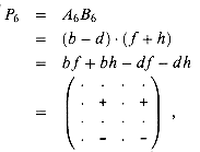
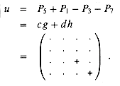
We can obtain u in a similar manner from P5 by using P1 and P3 to move the inessential terms of P5 in a different direction:
By subtracting an additional product
we now obtain
The 7 submatrix products P1, P2, . . . , P7 can thus be used to compute the product C = AB, which completes the description of Strassen's method.
The large constant hidden in the running time of Strassen's algorithm makes it impractical unless the matrices are large (n at least 45 or so) and dense (few zero entries). For small matrices, the straightforward algorithm is preferable, and for large, sparse matrices, there are special sparsematrix algorithms that beat Strassen's in practice. Thus, Strassen's method is largely of theoretical interest.
By using advanced techniques beyond the scope of this text, one can in fact multiply n
Strassen's algorithm does not require that the matrix entries be real numbers. All that matters is that the number system form an algebraic ring. If the matrix entries do not form a ring, however, sometimes other techniques can be brought to bear to allow his method to apply. These issues are discussed more fully in the next section.
31.2-1
Use Strassen's algorithm to compute the matrix product
Show your work.
31.2-2
How would you modify Strassen's algorithm to multiply n
31.2-3
What is the largest k such that if you can multiply 3
31.2-4
V. Pan has discovered a way of multiplying 68
131.2-5
How quickly can you multiply a kn
31.2-6
Show how to multiply the complex numbers a + bi and c + di using only three real multiplications. The algorithm should take a, b, c, and d as input and produce the real component ac - bd and the imaginary component ad + bc separately.
The properties of matrix addition and multiplication depend on the properties of the underlying number system. In this section, we define three different kinds of underlying number systems: quasirings, rings, and fields. We can define matrix multiplication over quasirings, and Strassen's matrix-multiplication algorithm works over rings. We then present a simple trick for reducing boolean matrix multiplication, which is defined over a quasiring that is not a ring, to multiplication over a ring. Finally, we discuss why the properties of a field cannot naturally be exploited to provide better algorithms for matrix multiplication.
Let
1.
Likewise,
2.
3. The operator
4. The operator
Examples of quasirings include the boolean quasiring ({0,1},
We can extend
Theorem 31.7
If
Proof The proof is left as Exercise 31.3-3.
Subtraction is not defined for quasirings, but it is for a ring, which is a quasiring
5. Every element in S has an additive inverse; that is, for all a
Given that the negative of any element is defined, we can define subtraction by a - b = a + (-b).
There are many examples of rings. The integers (Z, +,
The following corollary shows that Theorem 31.7 generalizes naturally to rings.
Corollary 31.8
If
Proof The proof is left as Exercise 31.3-3.
Using this corollary, we can prove the following theorem.
Theorem 31.9
Strassen's matrix-multiplication algorithm works properly over any ring of matrix elements.
Proof Strassen's algorithm depends on the correctness of the algorithm for 2
Strassen's algorithm for matrix multiplication, in fact, depends critically on the existence of additive inverses. Out of the seven products P1, P2, . . . ,P7, four involve differences of submatrices. Thus, Strassen's algorithm does not work in general for quasirings.
Strassen's algorithm cannot be used directly to multiply boolean matrices, since the boolean quasiring ({0,1},
The following theorem presents a simple trick for reducing boolean matrix multiplication to multiplication over a ring. Problem 31-1 presents another efficient approach.
Theorem 31.10
If M(n) denotes the number of arithmetic operations required to multiply two n
Proof Let the two matrices be A and B, and let C = AB in the boolean quasiring, that is,
Instead of computing over the boolean quasiring, we compute the product C' over the ring of integers with the given matrix-multiplication algorithm that uses M(n) arithmetic operations. We thus have
Each term aikbkj of this sum is 0 if and only if aik
Thus, using Strassen's algorithm, we can perform boolean matrix multiplication in O(n lg 7) time.
The normal method of multiplying boolean matrices uses only boolean variables. If we use this adaptation of Strassen's algorithm, however, the final product matrix can have entries as large as n, thus requiring a computer word to store them rather than a single bit. More worrisome is that the intermediate results, which are integers, may grow even larger. One method for keeping intermediate results from growing too large is to perform all computations modulo n + 1. Exercise 31.3-5 asks you to show that working modulo n + 1 does not affect the correctness of the algorithm.
A ring
6. The operator
7. Every nonzero element in S has a multiplicative inverse; that is, for all
Such an element b is often called the inverse of a and is denoted a-1.
Examples of fields include the real numbers (R, +,
Because fields offer multiplicative inverses of elements, division is possible. They also offer commutativity. By generalizing from quasirings to rings, Strassen was able to improve the running time of matrix multiplication. Since the underlying elements of matrices are often from a field--the real numbers, for instance--one might hope that by using fields instead of rings in a Strassen-like recursive algorithm, the running time might be further improved.
This approach seems unlikely to be fruitful. For a recursive divide-and-conquer algorithm based on fields to work, the matrices at each step of the recursion must form a field. Unfortunately, the natural extension of Theorem 31.7 and Corollary 31.8 to fields fails badly. For n > 1, the set of n
31.3-1
Does Strassen's algorithm work over the number system (Z[x], +,
31.3-2
Explain why Strassen's algorithm doesn't work over closed semirings (see Section 26.4) or over the boolean quasiring ({0, 1},
31.3-3
Prove Theorem 31.7 and Corollary 31.8.
31.3-4
Show that the boolean quasiring ({0, 1},
31.3-5
Argue that if all computations in the algorithm of Theorem 31.10 are performed modulo n + 1, the algorithm still works correctly.
31.3-6
Show how to determine efficiently if a given undirected input graph contains a triangle (a set of three mutually adjacent vertices).
31.3-7
Show that computing the product of two n
31.3-8
Show how to compute the transitive closure of a given directed n-vertex input graph in time O(nlg 7 lg n). Compare this result with the performance of the TRANSITIVE-CLOSURE procedure in Section 26.2.
Solving a set of simultaneous linear equations is a fundamental problem that occurs in diverse applications. A linear system can be expressed as a matrix equation in which each matrix or vector element belongs to a field, typically the real numbers R. This section discusses how to solve a system of linear equations using a method called LUP decomposition.
We start with a set of linear equations in n unknowns x1, x2, . . . , xn:
A set of values for x1, x2, . . . , xn that satisfy all of the equations (31.17) simultaneously is said to be a solution to these equations. In this section, we only treat the case in which there are exactly n equations in n unknowns.
We can conveniently rewrite equations (31.17) as the matrix-vector equation
or, equivalently, letting A = (aij), x = (xj), and b = (bi), as
If A is nonsingular, it possesses an inverse A-1, and
is the solution vector. We can prove that x is the unique solution to equation (31.18) as follows. If there are two solutions, x and x', then Ax = Ax' = b and
In this section, we shall be concerned predominantly with the case in which A is nonsingular or, equivalently (by Theorem 31.1), the rank of A is equal to the number n of unknowns. There are other possibilities, however, which merit a brief discussion. If the number of equations is less than the number n of unknowns--or, more generally, if the rank of A is less than n--then the system is underdetermined. An underdetermined system typically has infinitely many solutions (see Exercise 31.4-9), although it may have no solutions at all if the equations are inconsistent. If the number of equations exceeds the number n of unknowns, the system is overdetermined, and there may not exist any solutions. Finding good approximate solutions to overdetermined systems of linear equations is an important problem that is addressed in Section 31.6.
Let us return to our problem of solving the system Ax = b of n equations in n unknowns. One approach is to compute A-1 and then multiply both sides by A-1, yielding A-1Ax = A-1b, or x = A-1b. This approach suffers in practice from numerical instability: round-off errors tend to accumulate unduly when floating-point number representations are used instead of ideal real numbers. There is, fortunately, another approach--LUP decomposition--that is numerically stable and has the further advantage of being about a factor of 3 faster.
The idea behind LUP decomposition is to find three n
where
We call matrices L, U, and P satisfying equation (31.20) an LUP decomposition of the matrix A. We shall show that every nonsingular matrix A possesses such a decomposition.
The advantage of computing an LUP decomposition for the matrix A is that linear systems can be solved more readily when they are triangular, as is the case for both matrices L and U. Having found an LUP decomposition for A, we can solve the equation (31.18) Ax = b by solving only triangular linear systems, as follows. Multiplying both sides of Ax = b by P yields the equivalent equation P Ax = Pb, which by Exercise 31.1-2 amounts to permuting the equations (31.17). Using our decomposition (31.20), we obtain
We can now solve this equation by solving two triangular linear systems. Let us define y = Ux, where x is the desired solution vector. First, we solve the lower-triangular system
for the unknown vector y by a method called "forward substitution." Having solved for y, we then solve the upper-triangular system
for the unknown x by a method called "back substitution." The vector x is our solution to Ax = b, since the permutation matrix P is invertible (Exercise 31.1 -2):
Our next step is to show how forward and back substitution work and then attack the problem of computing the LUP decomposition itself.
Forward substitution can solve the lower-triangular system (31.21) in
Quite apparently, we can solve for y1 directly, since the first equation tells us that y1 = b
Now, we can substitute both y1 and y2 into the third equation, obtaining
In general, we substitute y1, y2, . . . ,yi-1 "forward" into the ith equation to solve for yi:
Back substitution is similar to forward substitution. Given U and y, we solve the nth equation first and work backward to to the first equation. Like forward substitution, this process runs in
Thus, we can solve for xn, xn-1, . . . , x1 successively as follows:
or, in general,
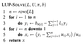
Given P, L, U, and b, the procedure LUP-SOLVE solves for x by combining forward and back substitution. The pseudocode assumes that the dimension n appears in the attribute rows[L] and that the permutation matrix P is represented by the array
Procedure LUP-SOLVE solves for y using forward substitution in lines 2-3, and then it solves for x using backward substitution in lines 4-5. Since there is an implicit loop in the summations within each of the for loops, the running time is
As an example of these methods, consider the system of linear equations defined by
where
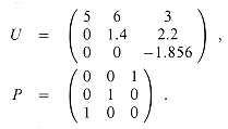
and we wish to solve for the unknown x. The LUP decomposition is
(The reader can verify that PA = LU.) Using forward substitution, we solve Ly = Pb for y:
obtaining
by computing first y1, then y2, and finally y3. Using back substitution, we solve Ux = y for x:
thereby obtaining the desired answer
by computing first x3, then x2, and finally x1.
We have now shown that if an LUP decomposition can be computed for a nonsingular matrix A, forward and back substitution can be used to solve the system Ax = b of linear equations. It remains to show how an LUP decomposition for A can be found efficiently. We start with the case in which A is an n
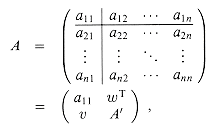
The process by which we perform LU decomposition is called Gaussian elimination. We start by subtracting multiples of the first equation from the other equations so that the first variable is removed from those equations. Then, we subtract multiples of the second equation from the third and subsequent equations so that now the first and second variables are removed from them. We continue this process until the system that is left has an upper-triangular form--in fact, it is the matrix U. The matrix L is made up of the row multipliers that cause variables to be eliminated.
Our algorithm to implement this strategy is recursive. We wish to construct an LU decomposition for an n
where v is a size-(n - 1) column vector, wT is a size-(n - 1) row vector, and A' is an (n - 1)
The 0's in the first and second matrices of the factorization are row and column vectors, respectively, of size n - 1. The term vwT/a11, formed by taking the outer product of v and w and dividing each element of the result by a11, is an (n - 1)
is called the Schur complement of A with respect to a11.
We now recursively find an LU decomposition of the Schur complement. Let us say that
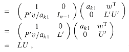
where L' is unit lower-triangular and U' is upper-triangular. Then, using matrix algebra, we have
thereby providing our LU decomposition. (Note that because L' is unit lower-triangular, so is L, and because U'is upper-triangular, so is U.)
Of course, if a11 = 0, this method doesn't work, because it divides by 0. It also doesn't work if the upper leftmost entry of the Schur complement A' - vwT/a11 is 0, since we divide by it in the next step of the recursion. The elements by which we divide during LU decomposition are called pivots, and they occupy the diagonal elements of the matrix U. The reason we include a permutation matrix P during LUP decomposition is that it allows us to avoid dividing by zero elements. Using permutations to avoid division by 0 (or by small numbers) is called pivoting.
An important class of matrices for which LU decomposition always works correctly is the class of symmetric positive-definite matrices. Such matrices require no pivoting, and thus the recursive strategy outlined above can be employed without fear of dividing by 0. We shall prove this result, as well as several others, in Section 31.6.
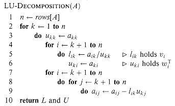
Our code for LU decomposition of a matrix A follows the recursive strategy, except that an iteration loop replaces the recursion. (This transformation is a standard optimization for a "tail-recursive" procedure--one whose last operation is a recursive call to itself.) It assumes that the dimension of A is kept in the attribute rows[A]. Since we know that the output matrix U has 0's below the diagonal, and since LU-SOLVE does not look at these entries, the code does not bother to fill them in. Likewise, because the output matrix L has 1's on its diagonal and 0's above the diagonal, these entries are not filled in either. Thus, the code computes only the "significant" entries of L and U.
The outer for loop beginning in line 2 iterates once for each recursive step. Within this loop, the pivot is determined to be ukk = akk in line 3. Within the for loop in lines 4-6 (which does not execute when k = n), the v and wT vectors are used to update L and U. The elements of the v vector are determined in line 5, where vi is stored in lik, and the elements of the wT vector are determined in line 6, where wiT is stored in uki. Finally, the elements of the Schur complement are computed in lines 7-9 and stored back in the matrix A. Because line 9 is triply nested, LU-DECOMPOSITION runs in time
Figure 31.1 illustrates the operation of LU-DECOMPOSITION. It shows a standard optimization of the procedure in which the significant elements of L and U are stored "in place" in the matrix A. That is, we can set up a correspondence between each element aij and either lij (if i > j) or uij (if i
Generally, in solving a system of linear equations Ax = b, we must pivot on off-diagonal elements of A to avoid dividing by 0. Not only is division by 0 undesirable, so is division by any small value, even if A is nonsingular, because numerical instabilities can result in the computation. We therefore try to pivot on a large value.
The mathematics behind LUP decomposition is similar to that of LU decomposition. Recall that we are given an n
where v = (a21, a31, . . . , an1)T, except that a11 replaces ak1; wT = (ak2, ak3, . . . , akn); and A' is an (n - 1)
The Schur complement A' - vwT/ak1 is nonsingular, because otherwise the second matrix in the last equation has determinant 0, and thus the determinant of matrix A is 0; but this means that A is singular, which contradicts our assumption that A is nonsingular. Consequently, we can inductively find an LUP decomposition for the Schur complement, with unit lower-triangular matrix L', upper-triangular matrix U', and permutation matrix P', such that
Define
which is a permutation matrix, since it is the product of two permutation matrices (Exercise 31.1-2). We now have
yielding the LUP decomposition. Because L' is unit lower-triangular, so is L, and because U' is upper-triangular, so is U.
Notice that in this derivation, unlike the one for LU decomposition, both the column vector v/ak1 and the Schur complement A' - vwT/ak1 must be multiplied by the permutation matrix P'.
Like LU-DECOMPOSITION, our pseudocode for LUP decomposition replaces the recursion with an iteration loop. As an improvement over a direct implementation of the recursion, we dynamically maintain the permutation matrix P as an array
Figure 31.2 illustrates how LUP-DECOMPOSITION factors a matrix. The array
If all elements in the current first column are zero, lines 10-11 report that the matrix is singular. To pivot, we exchange
Because of its triply nested loop structure, the running time of LUP-DECOMPOSITION is
31.4-1
Solve the equation
by using forward substitution.
31.4-2
Find an LU decomposition of the matrix
31.4-3
Why does the for loop in line 4 of LUP-DECOMPOSITION run only up to n - 1, whereas the corresponding for loop in line 2 of LU-DECOMPOSITION runs all the way to n?
31.4-4
Solve the equation
by using an LUP decomposition.
31.4-5
Describe the LUP decomposition of a diagonal matrix.
31.4-6
Describe the LUP decomposition of a permutation matrix A, and prove that it is unique.
31.4-7
Show that for all n
31.4-8
Show how we can efficiently solve a set of equations of the form Ax = b over the boolean quasiring ({0, 1},
31.4-9
Suppose that A is an m
Although in practice we do not generally use matrix inverses to solve systems of linear equations, preferring instead to use more numerically stable techniques such as LUP decomposition, it is sometimes necessary to compute a matrix inverse. In this section, we show how LUP decomposition can be used to compute a matrix inverse. We also discuss the theoretically interesting question of whether the computation of a matrix inverse can be sped up using techniques such as Strassen's algorithm for matrix multiplication. Indeed, Strassen's original paper was motivated by the problem of showing that a set of a linear equations could be solved more quickly than by the usual method.
Suppose that we have an LUP decomposition of a matrix A in the form of three matrices L, U, and P such that PA = LU. Using LU-SOLVE, we can solve an equation of the form Ax = b in time
The equation
can be viewed as a set of n distinct equations of the form Ax = b. These equations define the matrix X as the inverse of A. To be precise, let Xi denote the ith column of X, and recall that the unit vector ei is the ith column of In. Equation (31.24) can then be solved for X by using the LUP decomposition for A to solve each equation
separately for Xi. Each of the n Xi can be found in time
We now show that the theoretical speedups obtained for matrix multiplication translate to speedups for matrix inversion. In fact, we prove something stronger: matrix inversion is equivalent to matrix multiplication, in the following sense. If M(n) denotes the time to multiply two n
Theorem 31.11
If we can invert an n
Proof Let A and B be n
The inverse of D is
and thus we can compute the product AB by taking the upper right n
We can construct matrix D in
Note that I(n) satisfies the regularity condition whenever I(n) does not have large jumps in value. For example, if I(n) =
The proof that matrix inversion is no harder than matrix multiplication relies on some properties of symmetric positive-definite matrices that will be proved in Section 31.6.
Theorem 31.12
If we can multiply two n
Proof We can assume that n is an exact power of 2, since we have
for any k > 0. Thus, by choosing k such that n + k is a power of 2, we enlarge the matrix to a size that is the next power of 2 and obtain the desired answer A-1 from the answer to the enlarged problem. The regularity condition on M(n) ensures that this enlargement does not cause the running time to increase by more than a constant factor.
For the moment, let us assume that the n
Then, if we let
be the Schur complement of A with respect to B, we have
since AA-1 = In, as can be verified by performing the matrix multiplication. The matrices B-1 and S-1 exist if A is symmetric and positive-definite, by Lemmas 31.13, 31.14, and 31.15 in Section 31.6, because both B and S are symmetric and positive-definite. By Exercise 31.1-3, B-1CT = (CB-1)T and B-1CTS-1 = (S-1 CB-1)T. Equations (31.26) and (31.27) can therefore be used to specify a recursive algorithm involving 4 multiplications of n/2
Since we can multiply n/2
It remains to prove that the asymptotic running time of matrix multiplication can be obtained for matrix inversion when A is invertible but not symmetric and positive-definite. The basic idea is that for any nonsingular matrix A, the matrix ATA is symmetric (by Exercise 31.1-3) and positive-definite (by Theorem 31.6). The trick, then, is to reduce the problem of inverting A to the problem of inverting ATA.
The reduction is based on the observation that when A is an n
since ((ATA)-1 AT)A = (ATA)-1(ATA) = In and a matrix inverse is unique. Therefore, we can compute A-1 by first multiplying AT by A to obtain ATA, then inverting the symmetric positive-definite matrix ATA using the above divide-and-conquer algorithm, and finally multiplying the result by AT. Each of these three steps takes O(M(n)) time, and thus any nonsingular matrix with real entries can be inverted in O(M(n)) time.
The proof of Theorem 31.12 suggests a means of solving the equation Ax = b without pivoting, so long as A is nonsingular. We multiply both sides of the equation by AT, yielding (ATA)x = ATb. This transformation doesn't affect the solution x, since AT is invertible, so we can factor the symmetric positive-definite matrix ATA by computing an LU decomposition. We then use forward and back substitution to solve for x with the right-hand side ATb. Although this method is theoretically correct, in practice the procedure LUP-DECOMPOSITION works much better. LUP decomposition requires fewer arithmetic operations by a constant factor, and it has somewhat better numerical properties.
31.5-1
Let M(n) be the time to multiply n
31.5-2
Let M(n) be the time to multiply n
31.5-3
Let M(n) be the time to multiply n 

(31.2)
 1 matrix; the corresponding row vector is obtained by taking the transpose:
xT = ( 2 3 5 ) .
 n matrices arise frequently. Several special cases of square matrices are of particular interest:
 j. Because all of the off-diagonal elements are zero, the matrix can be specified by listing the elements along the diagonal:
 n identity matrix In is a diagonal matrix with 1's along the diagonal:
In = diag(1,1,...,1)



Operations on matrices
 n matrices, then their matrix sum C = (cij) = A + B is the m
  n matrix defined by
cij = aij + bij
A + 0 = A
= 0 + A .
 is a number and A = (aij) is a matrix, then
  A = (
A = ( aij) is the scalar multiple of A obtained by multiplying each of its elements by
  . As a special case, we define the negative of a matrix A = (aij) to be -1
  A = - A, so that the ijth entry of - A is -aij. Thus,
A + (-A) = 0
= (-A) + A .
 n matrix and B = (bjk) is an n
  p matrix, then their matrix product C = AB is the m
  p matrix C = (cik), where
(31.3)
 n matrices, MATRIX-MULTIPLY performs n3 multiplications and n2(n - 1) additions, and its running time is
  (n3).
(n3).ImA = AIn = A
 n matrix A. Multiplying by a zero matrix gives a zero matrix:
A 0 = 0 .
A(BC) = (AB)C
(31.4)
A(B + C) = AB + AC ,
(B + C)D = BD + CD .
(31.5)
 n matrices is not commutative, however, unless n = 1. For example, if
  and
and  , then

 1 matrix (or a 1
  n matrix, in the case of a row vector). Thus, if A is an m
  n matrix and x is a vector of size n, then Ax is a vector of size m. If x and y are vectors of size n, then
 1 matrix) called the inner product of x and y. The matrix xyT is an n
  n matrix Z called the outer product of x and y, with zij = xiyj. The (euclidean) norm ||x|| of a vector x of size n is defined by
Matrix inverses, ranks, and determinants
 n matrix A to be the n
  n matrix, denoted A-1 (if it exists), such that AA-1 = In = A-1 A. For example,
 n matrices do not have inverses. A matrix without an inverse is is called noninvertible, or singular. An example of a nonzero singular matrix is
 n matrices, then
(BA)-1 = A-1B-1.
(31.6)
(A-1)T = (AT)-1 .
 n matrix A is the size of the largest set of linearly independent columns of A. Similarly, the row rank of A is the size of the largest set of linearly independent rows of A. A fundamental property of any matrix A is that its row rank always equals its column rank, so that we can simply refer to the rank of A. The rank of an m
  n matrix is an integer between 0 and min(m, n), inclusive. (The rank of a zero matrix is 0, and the rank of an n
  n identity matrix is n.) An alternate, but equivalent and often more useful, definition is that the rank of a nonzero m
  n matrix A is the smallest number r such that there exist matrices B and C of respective sizes m
  r and r
  n such that
A = BC .
 n matrix has full rank if its rank is n. A fundamental property of ranks is given by the following theorem.
 n matrix has full column rank if its rank is n.
 n matrix A, for n > 1, is the (n - 1)
  (n - 1) matrix A[ij] obtained by deleting the ith row and jth column of A. The determinant of an n
  n matrix A can be defined recursively in terms of its minors by
(31.7)
 If any row or any column of A is zero, then det (A) = 0.
 The determinant of A is multiplied by
  if the entries of any one row (or any one column) of A are all multiplied by
  .
. The determinant of A is unchanged if the entries in one row (respectively, column) are added to those in another row (respectively, column).
 The determinant of A equals the determinant of AT.
 The determinant of A is multiplied by - 1 if any two rows (respectively, columns) are exchanged.
 n matrix A is singular if and only if det(A) = 0.
 Positive-definite matrices
 n matrix A is positive-definite if xT Ax > 0 for all size-n vectors x
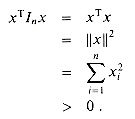
  0. For example, the identity matrix is positive-definite, since for any nonzero vector x = ( x1 x2 . . . xn)T,
xT(AT A)x = (Ax)T(Ax) (by Exercise 31.1-3)
= ||Ax||2
 0 .
0 .(31.8)
Exercises
 n permutation matrix and A is an n
  n matrix, then PA can be obtained from A by permuting its rows, and AP can be obtained from A by permuting its columns. Prove that the product of two permutation matrices is a permutation matrix. Prove that if P is a permutation matrix, then P is invertible, its inverse is PT, and PT is a permutation matrix.
 n matrices such that AB = I. Prove that if A' is obtained from A by adding row j into row i, then the inverse B' of A' can be obtained by subtracting column i from column j of B.
 n matrix with complex entries. Show that every entry of A-1 is real if and only if every entry of A is real.
 min(rank(A), rank(B)) ,

31.2 Strassen's algorithm for matrix multiplication
 n matrices that runs in
  (nlg 7) = O(n2.81) time. For sufficiently large n, therefore, it outperforms the naive
  (n3) matrix-multiplication algorithm MATRIX-MULTIPLY from Section 26.1.
An overview of the algorithm
 n matrices. Assuming that n is an exact power of 2, we divide each of A, B, and C into four n/2
  n/2 matrices, rewriting the equation C = AB as follows:
(31.9)
r = ae + bf ,
(31.10)
s = ag + bh ,
(31.11)
t = ce + df ,
(31.12)
u = cg + dh .
(31.13)
 n/2 matrices and the addition of their n/2
  n/2 products. Using these equations to define a straightforward divide-and-conquer strategy, we derive the following recurrence for the time T(n) to multiply two n
  n matrices:
T(n) = 8T(n/2) +
 (n2).
(n2).(31.14)
 (n3), and thus this method is no faster than the ordinary one.
 n/2 matrices and
  (n2) scalar additions and subtractions, yielding the recurrence
T(n) = 7T(n/2) +
 (n2)
(n2)=
 (nlg 7)
= O(n2.81) .
(31.15)
 n/2 submatrices, as in equation (31.9).
 (n2) scalar additions and subtractions, compute 14 n/2
  n/2 matrices A1, B1, A2, B2, . . . , A7, B7.
 (n2) scalar additions and subtractions.
Determining the submatrix products
Pi = AiBi
= (
 i1a +
i1a +  i2b +
i2b +  i3c +
i3c +  i4d)
i4d)  (
( i1e +
i1e +  i2f +
i2f +  i3g +
i3g +  i4h) ,
(31.16)
 ij,
ij,  ij are all drawn from the set {-1, 0, 1}. That is, we guess that each product is computed by adding or subtracting some of the submatrices of A, adding or subtracting some of the submatrices of B, and then multiplying the two results together. While more general strategies are possible, this simple one turns out to work.
 4 matrices to represent linear combinations of products of submatrices, where each product combines one submatrix of A with one submatrix of B as in equation (31.16). For example, we can rewrite equation (31.10) as

 represents 0, and "-" represents -1. (From here on, we omit the row and column labels.) Using this notation, we have the following equations for the other submatrices of the result matrix C:
Discussion
 n matrices in better than
  (n1g 7) time. The current best upper bound is approximately O(n2.376). The best lower bound known is just the obvious
  (n2) bound (obvious because we have to fill in n2 elements of the product matrix). Thus, we currently do not know how hard matrix multiplication really is.
Exercises

 n matrices in which n is not an exact power of 2? Show that the resulting algorithm runs in time
  (n1g 7).
 3 matrices using k multiplications (not assuming commutativity of multiplication), then you can multiply n
  n matrices in time o(n1g 7)? What would the running time of this algorithm be?
 68 matrices using 132,464 multiplications, a way of multiplying 70
  70 matrices using 143,640 multiplications, and a way of multiplying 72
  72 matrices using 155,424 multiplications. Which method yields the best asymptotic running time when used in a divide-and-conquer matrix-multiplication algorithm? Compare it with the running time for Strassen's algorithm.
 n matrix by an n
  kn matrix, using Strassen's algorithm as a subroutine? Answer the same question with the order of the input matrices reversed.
* 31.3 Algebraic number systems and boolean matrix multiplication
Quasirings
 denote a number system, where S is a set of elements,
  and
and  are binary operations on S (the addition and multiplication operations, respectively), and
  are distinct distinguished elements of S. This system is a quasiring if it satisfies the following properties:
 is a monoid:
 S is closed under
  ; that is, a
  b
b  S for all a, b
  S.
S.
 is associative; that is, a
  (b
(b  c) = (a
  b)
b)  c for all a, b, c
  S.
S.
 is an identity for
  ; that is,
  for all a
  S.
S. is a monoid.
 is an annihilator, that is,
  for all a
  S.
S. is commutative; that is, a
  b = b
b = b  a for all a, b
  S.
S. distributes over
  ; that is,
  and
and  for all a,b,c
  S.
S. ,
,  , 0, 1), where
  denotes logical OR and
  denotes logical AND, and the natural number system (N, +,
  , 0, 1), where + and
  denote ordinary addition and multiplication. Any closed semiring (see Section 26.4) is also a quasiring; closed semirings obey additional idempotence and infinite-sum properties.
 and
and  to matrices as we did for + and
  in Section 31.1. Denoting the n
  n identity matrix composed of
  we find that matrix multiplication is well defined and the matrix system is itself a quasiring, as the following theorem states.
 is a quasiring and n
  1, then
  is a quasiring.
Rings
 that satisfies the following additional property:
 S, there exists an element b
  S such that
  . Such a b is also called the negative of a and is denoted (-a).
 , 0, 1) under the usual operations of addition and multiplication form a ring. The integers modulo n for any integer n > 1--that is, (Zn, +,
  , 0, 1), where + is addition modulo n and
  is multiplication modulo n--form a ring. Another example is the set R[x] of finite-degree polynomials in x with real coefficients under the usual operations--that is, (R[x], +,
  , 0, 1), where + is polynomial addition and
  is polynomial multiplication.
 is a ring and n
  1, then
  is a ring.
 2 matrices, which requires only that the matrix elements belong to a ring. Since the matrix elements do belong to a ring, Corollary 31.8 implies the matrices themselves form a ring. Thus, by induction, Strassen's algorithm works correctly at each level of recursion.
 Boolean matrix multiplication
 ,
,  , 0, 1) is not a ring. There are instances in which a quasiring is contained in a larger system that is a ring. For example, the natural numbers (a quasiring) are a subset of the integers (a ring), and Strassen's algorithm can therefore be used to multiply matrices of natural numbers if we consider the underlying number system to be the integers. Unfortunately, the boolean quasiring cannot be extended in a similar way to a ring. (See Exercise 31.3-4.)
 n matrices over the integers, then two n
  n boolean matrices can be multiplied using O(M(n)) arithmetic operations.

 bkj = 0, and 1 if and only if aik
  bkj = 1. Thus, the integer sum
  is 0 if and only if every term is 0 or, equivalently, if and only if the boolean OR of the terms, which is cij, is 0. Therefore, the boolean matrix C can be reconstructed with
  (n2) arithmetic operations from the integer matrix C' by simply comparing each
  with 0. The number of arithmetic operations for the entire procedure is then O(M(n)) +
 (n2) = O(M(n)), since M(n) =
  (n2).
(n2). Fields
 is a field if it satisfies the following two additional properties:
 is commutative; that is,
  for all a, b
  S.
S. , there exists an element b
  S such that
  .
. , 0, 1), the complex numbers (C, +,
  , 0, 1), and the integers modulo a prime p: (Zp, +,
  , 0, 1).
 n matrices never forms a field, even if the underlying number system is a field. Multiplication of n
  n matrices is not commutative, and many n
  n matrices do not have inverses. Better algorithms for matrix multiplication are therefore more likely to be based on ring theory than on field theory.
Exercises
 , 0, 1), where Z[x] is the set of all polynomials with integer coefficients in the variable x and + and
  are ordinary polynomial addition and multiplication?
 ,
,  , 0, 1).
 ,
,  , 0, 1) cannot be embedded in a ring. That is, show that it is impossible to add a "-1" to the quasiring so that the resulting algebraic structure is a ring.
 n boolean matrices over the boolean quasiring is reducible to computing the transitive closure of a given directed 3n-vertex input graph.
31.4 Solving systems of linear equations
a11x1 + a12x2 +


 + a1nxn = b1,
a21x1 + a22x2 +


 + a2nxn = b2,
(31.17)
an1x1 + an2x2 +


 + annxn = bn.
Ax = b .
(31.18)
x = A-1 b
(31.19)
x = (A-1 A)x
= A-1(Ax)
= A-1(Ax')
= (A-1 A)x'
= x'.
Overview of LUP decomposition
 n matrices L, U, and P such that
PA = LU ,
(31.20)
 L is a unit lower-triangular matrix,
 U is an upper-triangular matrix, and
 P is a permutation matrix.
LUx = Pb .
Ly = Pb
(31.21)
Ux = y
(31.22)
Ax = P-1 LUx
= P-1 Ly
= P-1 Pb
= b .
Forward and back substitution
 (n2) time, given L, P, and b. For convenience, we represent the permutation P compactly by an array
  [1 . . n]. For i = 1, 2, . . . , n, the entry
  [i] indicates that Pi,
 [i] = 1 and Pij = 0 for j
 [i]. Thus, PA has a
 [i],j in row i and column j, and Pb has b
 [i] as its ith element. Since L is unit lower-triangular, equation (31.21) can be rewritten as
y1 = b
 [1],
[1],l21y1 + y2 = b
 [2],
[2],l31y1 + l32y2 + y3 = b
 [3],
[3],
ln1y1 + ln2y2 + ln3y3 +


 + yn = b
 [n].
[n]. [1]. Having solved for y1, we can substitute it into the second equation, yielding
y2 = b
 [2] - l21y1.
y3 = b
 [3] - (l31y1 + l32y2).
 (n2) time. Since U is upper-triangular, we can rewrite the system (31.22) as
u11x1 + u12x2 +


 + u1,n-2xn-2 + u1,n-1xn-1 + u1nxn = y1,
u22x2 +


 + u2,n-2xn-2 + u2,n-1xn-1 + u2nxn = y2,
un-2,n-2xn-2 + un-2,n-1xn-1 + un-2,nxn = yn-2,
un-1,n-1xn-1 + un-1,nxn = yn-1,
un,nxn = yn .
xn = yn/unn ,
xn-1 = (yn-1 - un-1,nxn)/un-1,n-1 ,
xn-2 = (yn-2 - (un-2,n-1xn-1 + un-2,nxn))/un-2,n-2 ,


 .
.
 (n2).
(n2).




Computing an LU decomposition
 n nonsingular matrix and P is absent (or, equivalently, P = In). In this case, we must find a factorization A = LU. We call the two matrices L and U an LU decomposition of A.
 n nonsingular matrix A. If n = 1, then we're done, since we can choose L = I1 and U = A. For n > 1, we break A into four parts:
 (n - 1) matrix. Then, using matrix algebra (verify the equations by simply multiplying through), we can factor A as
 (n - 1) matrix, which conforms in size to the matrix A' from which it is subtracted. The resulting (n - 1)
  (n - 1) matrix
A' - vwT/a11
(31.23)
A' - vwT/a11 = L'U' ,

 (n3).
(n3).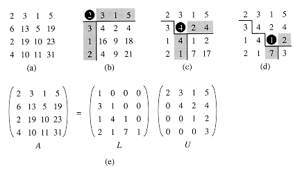
Figure 31.1 The operation of LU-DECOMPOSITION. (a) The matrix A. (b) The element a11 = 2 in black is the pivot, the shaded column is v/a11, and the shaded row is wT. The elements of U computed thus far are above the horizontal line, and the elements of L are to the left of the vertical line. The Schur complement matrix A' - vwT/a11 occupies the lower right. (c) We now operate on the Schur complement matrix produced from part (b). The element a22 = 4 in black is the pivot, and the shaded column and row are v/a22 and wT (in the partitioning of the Schur complement), respectively. Lines divide the matrix into the elements of U computed so far (above), the elements of L computed so far (left), and the new Schur complement (lower right). (d) The next step completes the factorization. (The element 3 in the new Schur complement becomes part of U when the recursion terminates.) (e) The factorization A = LU.
 j) and update the matrix A so that it holds both L and U when the procedure terminates. The pseudocode for this optimization is obtained from the above pseudocode merely by replacing each reference to l or u by a; it is not difficult to verify that this transformation preserves correctness.
Computing an LUP decomposition
 n nonsingular matrix A and wish to find a permutation matrix P, a unit lower-triangular matrix L, and an upper-triangular matrix U such that PA = LU. Before we partition the matrix A, as we did for LU decomposition, we move a nonzero element, say ak1, from the first column to the (1,1) position of the matrix. (If the first column contains only 0's, then A is singular, because its determinant is 0, by Theorems 31.4 and 31.5.) In order to preserve the set of equations, we exchange row 1 with row k, which is equivalent to multiplying A by a permutation matrix Q on the left (Exercise 31.1-2). Thus, we can write QA as
 (n - 1) matrix. Since ak1
  0, we can now perform much the same linear algebra as for LU decomposition, but now guaranteeing that we do not divide by 0:
P'(A' - vwT/ak1) = L'U' .


 , where
  [i] = j means that the ith row of P contains a 1 in column j. We also implement the code to compute L and U "in place" in the matrix A. Thus, when the procedure terminates,
LUP-DECOMPOSITION(A)
1 n
 rows[A]
2 for i
 1 to n
3 do
 [i]
[i]  i
i4 for k
 1 to n - 1
5 do p
 0
06 for i
 k to n
7 do if |aik| > p
8 then p
 |aik|
|aik|9 k'
 i
i10 if p = 0
11 then error "singular matrix"
12 exchange
 [k]
[k] 
 [k']
[k']13 for i
 1 to n
14 do exchange aki
 ak'i
ak'i15 for i
 k + 1 to n
16 do aik
 aik/akk
17 for j
 k + 1 to n
18 do aij
 aij - aikakj
 is initialized by lines 2-3 to represent the identity permutation. The outer for loop beginning in line 4 implements the recursion. Each time through the outer loop, lines 5-9 determine the element ak'k with largest absolute value of those in the current first column (column k) of the (n - k + l )
  (n - k + 1) matrix whose LU decomposition must be found.
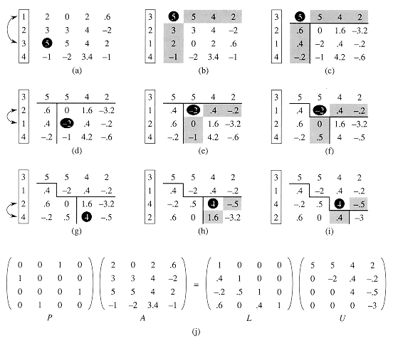
Figure 31.2 The operation of LUP-DECOMPOSITION. (a) The input matrix A with the identity permutation of the rows on the left. The first step of the algorithm determines that the element 5 in black in the third row is the pivot for the first column. (b) Rows 1 and 3 are swapped and the permutation is updated. The shaded column and row represent v and wT. (c) The vector v is replaced by v/5, and the the lower right of the matrix is updated with the Schur complement. Lines divide the matrix into three regions: elements of U (above), elements of L (left), and elements of the Schur complement (lower right).(d)-(f) The second step.(g)-(i) The third step finishes the algorithm. (j) The LUP decomposition PA = LU.
 [k'] with
  [k] in line 12 and exchange the kth and k'th rows of A in lines 13-14, thereby making the pivot element akk. (The entire rows are swapped because in the derivation of the method above, not only is A' - vwT/ak1 multiplied by P', but so is v/ak1.) Finally, the Schur complement is computed by lines 15-18 in much the same way as it is computed by lines 4-9 of LU-DECOMPOSITION, except that here the operation is written to work "in place."
 (n3), the same as that of LU-DECOMPOSITION. Thus, pivoting costs us at most a constant factor in time.
Exercises


 1, there exist singular n
  n matrices that have LU decompositions.
 ,
,  , 0, 1).
 n real matrix of rank m, where m < n. Show how to find a size-n vector x0 and an m
  (n - m) matrix B of rank n - m such that every vector of the form x0 + By, for y
  Rn-m, is a solution to the underdetermined equation Ax = b.
31.5 Inverting matrices
Computing a matrix inverse from an LUP decomposition
 (n2). Since the LUP decomposition depends on A but not b, we can solve a second set of equations of the form Ax = b' in additional time
  (n2). In general, once we have the LUP decomposition of A, we can solve, in time
  (kn2), k versions of the equation Ax = b that differ only in b.
AX = In
(31.24)
AXi = ei
 (n2), and so the computation of X from the LUP decomposition of A takes time
  (n3). Since the LUP decomposition of A can be computed in time
  (n3), the inverse A-1 of a matrix A can be determined in time
  (n3).
(n3).Matrix multiplication and matrix inversion
 n matrices and I(n) denotes the time to invert a nonsingular n
  n matrix, then I(n) =
  (M(n)). We prove this result in two parts. First, we show that M(n) = O(I(n)), which is relatively easy, and then we prove that I(n) = O(M(n)).
 n matrix in time I(n), where I(n) =
  (n2) and I(n) satisfies the regularity condition I(3n) = O(I(n)), then we can multiply two n
  n matrices in time O(I(n)).
 n matrices whose matrix product C we wish to compute. We define the 3n
  3n matrix D by

 n submatrix of D-1.
 (n2) = O(I(n)) time, and we can invert D in O(I(3n)) = O(I(n)) time, by the regularity condition on I(n). We thus have
M(n) = O(I(n)).
 (nc lgd n) for any constants c > 0, d
  0, then I(n) satisfies the regularity condition.
Reducing matrix inversion to matrix multiplication
 n real matrices in time M(n), where M(n) =
  (n2) and M(n) = O(M(n + k)) for 0
  k
k  n, then we can compute the inverse of any real nonsingular n
  n matrix in time O(M(n)).
 n matrix A is symmetric and positive-definite. We partition A into four n/2
  n/2 submatrices:
(31.25)
S = D - CB-1 CT
(31.26)

(31.27)
 n/2 matrices:
C
 B-1,
B-1,(CB-1)
 CT,
CT,S-1
 (CB-1),
(CB-1)T
 (S-1 CB-1).
 n/2 matrices using an algorithm for n
  n matrices, matrix inversion of symmetric positive-definite matrices can be performed in time
I(n)
 2I(n/2) + 4M(n) + O(n2)
= 2I(n/2) + O(M(n))
= O(M(n)).
 n nonsingular matrix, we have
A-1 = (ATA)-1AT,
Exercises
 n matrices, and let S(n) denote the time required to square an n
  n matrix. Show that multiplying and squaring matrices have essentially the same difficulty: S(n) =
  (M(n)).
 n matrices, and let L(n) be the time to compute the LUP decomposition of an n
  n matrix. Show that multiplying matrices and computing LUP decompositions of matrices have essentially the same difficulty: L(n) =
  (M(n)).
 n matrices, and let D(n) denote the time required to find the determinant of an n
  n matrix. Show that finding the determinant is no harder than multiplying matrices: D(n) = O(M(n)).


