Now that we have found our use cases and actors, it is time to start tackling the logical database design. We are going to use Object Role Modeling (ORM) to come up with our design. We will not show how we constructed all of this design, but we are going to show parts of it so you understand how you approach this process in real life.
Our users are placed in AD or ADAM as we stated earlier, so we do not have to consider them in our model. Instead, we are going to take a closer look at the report lines that belong to a user's weekly report. A line has information about the time type and number of hours worked on a project that the employee has spent time on during the week.
What we need to do first is find the objects that are participating in our model. The User is the first object we find. We know that users create user reports every week, so UserReport represents another object in our model. (We have also found a predicate here that we will need for our ORM model, but let us come back to this a bit later.) What else do we know? Well, every UserReport has one or more report lines. Hence we can make ReportLine another object. The objects are shown as ovals in the model as you can see by the example object in Figure 9-16.
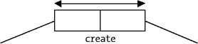
As we discussed in Chapter 1, objects are connected by predicates. These are portrayed as sequence boxes in a ORM model (see Figure 9-17). As we mentioned, we have already found a predicate for our example earlier.
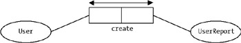
Referring back to "users create UserReport," you can see that the sequence box in this case is create. The predicate is the whole phrase "users create UserReport," and the box is only a role that exists within the predicate, as demonstrated in Figure 9-18.
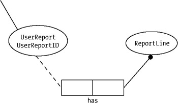
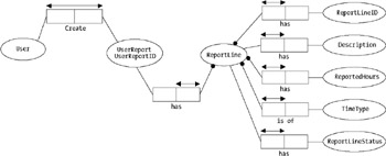
The next predicate we find is "UserReport has ReportLine." This is pretty obvious too, since we know a report is built up by one or more report lines. If we continue looking at objects and how they function, we can find many more predicates. The most relevant for this example are the following:
ReportLine has ReportLineID.
ReportLine has Description.
ReportLine has ReportedHours.
ReportLine is of TimeType.
ReportLine has ReportLineStatus.
The number of predicates all depends on the business requirements we have. The ones just listed serve our purposes, however, so we stop with these.
Some of the objects involved with ReportLine are unique. For example, a report line has only one ID. It can also only be of one time type and so on. We show this uniqueness with an arrow-tipped bar over the sequence box as you can see in Figure 9-19.
Next we see if we have any mandatory roles in our model. We show this as a dot on the connector. In our case, the report line ID is mandatory, as shown in Figure 9-20. We must have an identifier for the report line. We also find that reported hours, time type, and user report ID are mandatory.
We do not find any constraints in our model, however.
When we combine all of our findings to form a complete model, we end up with something similar to Figure 9-21.
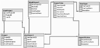
Now we are going to transform the ORM model into a logical database model. In it we are going to describe the ORM model in tables and columns instead of in sentences. Figure 9-22 shows how we have transformed our ORM model into a database schema.
By doing this, we make sure that read and write data gets locked as little as possible. We do not have to back up all historical data as often as we back up the current data. This speeds up backups.
As our database schema shows, we end up with seven tables:
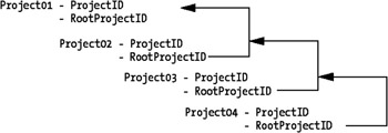
Project: Here all projects in the company will be stored. To allow any number of subprojects, we have a column called RootProjectID, which references ProjectID in the same table.
To simplify, you can think of this concept as illustrated in Figure 9-23. Recursive references will make a project like Project01 the root to Project02, which in turn will be the root project for Project03, and so on. This way we eliminate the need for a separate reference table.
UserProject: This table contains all the projects that are tied to a specific user. We keep track of them by the UserID.
WeekReport: This table simply keeps track of the weeks during a year. Each week's start and end date is entered as well as the expected number of hours an employee should work that week.
UserReport: This table holds all reports for a user. Even if a report has been rejected, the ReportStatus holds an ID for that report.
ReportLine: Here all the individual report lines for a UserReport are kept. The StatusID is filled only if the line has been rejected.
ReportStatus: A table that contains all status values that a report can have, such as submitted, rejected, saved, and so on.
TimeType: This table keeps track of the time types available to our users. Examples of this are normal hours, overtime, vacation, and so on.
Users: Although users are not stored in a table, as evidenced in Figure 9-22, we will remind you of them here anyway. As we said earlier, they will be fetched from AD or ADAM. All their information will be maintained in the directory.
Figure 9-22 also shows the relations between the tables. We have created one ID column for each table as well.
Before we start looking at how to index our database, we are going to consider the physical database design.
Our database server has four mapped drives from the SAN: E, F, G, and H. They all offer RAID 10 so we get both good read and write performance from these drives.
The log will be maintained in a single log file. It is always written to sequentially, so we do not benefit from splitting it up. We create it on drive E with a size of 100 megabytes. We also enable auto-growth in case our estimate is incorrect and the file needs to be expanded, as well as set a maximum value for the log file.
We will maintain the tables as follows:
The tables for the current and future weeks will be maintained in filegroup1 on drive F.
The tables for the current year will be maintained in filegroup2 on drive G.
The tables for the historical data will be maintained in filegroup3 on drive H.
All data files have auto-growth enabled and a maximum file size specified so they will not grow beyond control. As we stated earlier, we will partition the data horizontally. Since the current week is the only one being written to, we place it on a separate mapped drive. Managers will probably generate reports from the current year mostly, so we also place these on a separate drive. All other historical data will be maintained on yet another drive. The benefits of this setup are as follows:
Write operations are fast.
Read operations lock write operations as little as possible.
Backups can be taken of the filegroups separately, enabling us to implement a different backup strategy for each group. This way we do not need to back up the historical data as often as we back up the rest of the data. This will increase performance on backups.
A restoration of the database can be done on separate filegroups, which increases restoration performance.
At this point we can start planning our indexes. We do this by looking at each table and estimate how it will be accessed. Which columns will be used most frequently in the WHERE clauses of SELECT statements must be considered, and so on. Table 9-2 shows our first estimates. After that we will have to monitor the application and see if we need to change anything, first in the lab, and then in production.
|
Table |
Indexes |
|---|---|
|
Project |
Clustered on ProjectID, nonclustered on ProjectName and RootProjectID |
|
ReportLine |
Clustered on ReportID and ReportLineID |
|
ReportStatus |
Clustered on ReportStatusID |
|
UserProject |
Clustered on UserID and ProjectID, nonclustered on UseProjectID |
|
UserReport |
Clustered on UserID and WeekReportID |
|
WeekReport |
Clustered on WeekNumber |