


It is appropriate that we begin our study of data structures with the array. The array is often the only means for structuring data which is provided in a programming language. Therefore it deserves a significant amount of attention. If one asks a group of programmers to define an array, the most often quoted saying is: a consecutive set of memory locations. This is unfortunate because it clearly reveals a common point of confusion, namely the distinction between a data structure and its representation. It is true that arrays are almost always implemented by using consecutive memory, but not always. Intuitively, an array is a set of pairs, index and value. For each index which is defined, there is a value associated with that index. In mathematical terms we call this a correspondence or a mapping. However, as computer scientists we want to provide a more functional definition by giving the operations which are permitted on this data structure. For arrays this means we are concerned with only two operations which retrieve and store values. Using our notation this object can be defined as:
The function CREATE produces a new, empty array. RETRIEVE takes as input an array and an index, and either returns the appropriate value or an error. STORE is used to enter new index-value pairs. The second axiom is read as "to retrieve the j-th item where x has already been stored at index i in A is equivalent to checking if i and j are equal and if so, x, or search for the j-th value in the remaining array, A." This axiom was originally given by J. McCarthy. Notice how the axioms are independent of any representation scheme. Also, i and j need not necessarily be integers, but we assume only that an EQUAL function can be devised.
If we restrict the index values to be integers, then assuming a conventional random access memory we can implement STORE and RETRIEVE so that they operate in a constant amount of time. If we interpret the indices to be n-dimensional, (i1,i2, ...,in), then the previous axioms apply immediately and define n-dimensional arrays. In section 2.4 we will examine how to implement RETRIEVE and STORE for multi-dimensional arrays using consecutive memory locations.
One of the simplest and most commonly found data object is the ordered or linear list. Examples are the days of the week
(MONDAY, TUESDAY, WEDNESDAY, THURSDAY, FRIDAY,
SATURDAY, SUNDAY)
or the values in a card deck
(2, 3, 4, 5, 6, 7, 8, 9, 10, Jack, Queen, King, Ace)
or the floors of a building
(basement, lobby, mezzanine, first, second, third)
or the years the United States fought in World War II
(1941, 1942, 1943, 1944, 1945).
If we consider an ordered list more abstractly, we say that it is either empty or it can be written as
(a1,a2,a3, ...,an)
where the ai are atoms from some set S.
There are a variety of operations that are performed on these lists. These operations include:
(i) find the length of the list, n;
(ii) read the list from left-to-right (or right-to-left);
(iii) retrieve the i-th element,
(iv) store a new value into the i-th position,
(v) insert a new element at position
(vi) delete the element at position
See exercise 24 for a set of axioms which uses these operations to abstractly define an ordered list. It is not always necessary to be able to perform all of these operations; many times a subset will suffice. In the study of data structures we are interested in ways of representing ordered lists so that these operations can be carried out efficiently.
Perhaps the most common way to represent an ordered list is by an array where we associate the list element ai with the array index i. This we will refer to as a sequential mapping, because using the conventional array representation we are storing ai and ai + 1 into consecutive locations i and i + 1 of the array. This gives us the ability to retrieve or modify the values of random elements in the list in a constant amount of time, essentially because a computer memory has random access to any word. We can access the list element values in either direction by changing the subscript values in a controlled way. It is only operations (v) and (vi) which require real effort. Insertion and deletion using sequential allocation forces us to move some of the remaining elements so the sequential mapping is preserved in its proper form. It is precisely this overhead which leads us to consider nonsequential mappings of ordered lists into arrays in Chapter 4.
Let us jump right into a problem requiring ordered lists which we will solve by using one dimensional arrays. This problem has become the classical example for motivating the use of list processing techniques which we will see in later chapters. Therefore, it makes sense to look at the problem and see why arrays offer only a partially adequate solution. The problem calls for building a set of subroutines which allow for the manipulation of symbolic polynomials. By "symbolic," we mean the list of coefficients and exponents which accompany a polynomial, e.g. two such polynomials are
A(x) = 3x2 + 2x + 4 and B(x) = x4 + 10x3 + 3x2 + 1
For a start, the capabilities we would include are the four basic arithmetic operations: addition, subtraction, multiplication, and division. We will also need input and output routines and some suitable format for preparing polynomials as input. The first step is to consider how to define polynomials as a computer structure. For a mathematician a polynomial is a sum of terms where each term has the form axe; x is the variable, a is the coefficient and e is the exponent. However this is not an appropriate definition for our purposes. When defining a data object one must decide what functions will be available, what their input is, what their output is and exactly what it is that they do. A complete specification of the data structure polynomial is now given.
In this specification every polynomial is either ZERO or constructed by applying ATTACH to a polynomial. For example the polynomial P = 10x - 12x3 - 10x + 0x2 is represented by the string
ATTACH(ATTACH(ATTACH(ATTACH(ZERO, 10,1),-12,3),
- 10,1),0,2).
Notice the absense of any assumptions about the order of exponents, about nonzero coefficients, etc. These assumptions are decisions of representation. Suppose we wish to remove from P those terms having exponent one. Then we would write REM(P, 1) and by the axioms the above string would be transformed into
ATTACH(REM(ATTACH(ATTACH(ATTACH(ZERO,10,1), - 12,3),
- 10,1),1),0,2)
which is transformed into
ATTACH(REM(ATTACH(ATTACH(ZERO,10,1), - 12,3),1),0,2)
which becomes
ATTACH(ATTACH(REM(ATTACH(ZERO,10,1),1) - 12,3),0,2)
which becomes
ATTACH(ATTACH(REM(ZERO,1), - 12,3),0,2)
which becomes finally
ATTACH(ATTACH(ZERO, - 12,3),0,2)
or - 12x3 + 0x2.
These axioms are valuable in that they describe the meaning of each operation concisely and without implying an implementation. Note how trivial the addition and multiplication operations have become.
Now we can make some representation decisions. Exponents should be unique and in decreasing order is a very reasonable first decision. This considerably simplifies the operations ISZERO, COEF and REM while ADD, SMULT and MULT remain unchanged. Now assuming a new function EXP (poly)
insert any remaining terms in A or B into C
The basic loop of this algorithm consists of merging the terms of the two polynomials, depending upon the result of comparing the exponents. The case statement determines how the exponents are related and performs the proper action. Since the tests within the case statement require two terms, if one polynomial gets exhausted we must exit and the remaining terms of the other can be copied directly into the result. With these insights, suppose we now consider the representation question more carefully.
A general polynomial A(x) can be written as
anxn + an-1xn-1 + ... + a1x + a0
where an
A = (n,an ,an-1, ...,a1,a0).
The first element is the degree of A followed by the n + 1 coefficients in order of decreasing exponent. This representation leads to very simple algorithms for addition and multiplication. We have avoided the need to explicitly store the exponent of each term and instead we can deduce its value by knowing our position in the list and the degree.
But are there any disadvantages to this representation? Hopefully you have already guessed the worst one, which is the large amount of wasted storage for certain polynomials. Consider x1000 + 1, for instance. It will require a vector of length 1002, while 999 of those values will be zero. Therefore, we are led to consider an alternative scheme.
Suppose we take the polynomial A(x) above and keep only its nonzero coefficients. Then we will really have the polynomial
bm-1 xem-1 + bm-2xem-2 + ... + boxeo
where each bi is a nonzero coefficient of A and the exponents ei are decreasing
(m,em-1,bm-1,em-2,bm-2, ...,e0,b0).
The first entry is the number of nonzero terms. Then for each term there are two entries representing an exponent-coefficient pair.
Is this method any better than the first scheme? Well, it certainly solves our problem with x1000 + 1, which now would be represented as (2,1000,1,0,1). Basic algorithms will need to be more complex because we must check each exponent before we handle its coefficient, but this is not too serious. As for storage, this scheme could be worse than the former. For example, x4 + 10x3 + 3x2 + 1 would have the two forms
(4,1,10,3,0,1) or (4,4,1,3,10,2,3,0,1).
In the worst case, scheme 2 requires less than twice as much storage as scheme 1 (when the degree = n and all n + 1 coefficients are nonzero). But scheme 1 could be much more wasteful, as in the case of x1000 + 1, where it needs more than 200 times as many locations. Therefore, we will prefer representation scheme 2 and use it.
Let us now write a procedure in SPARKS for adding two polynomials represented as in scheme 2.
As this is one of our first complex algorithms written in SPARKS, suppose we point out some features. The procedure has parameters which are polynomial (or array) names, and hence they are capitalized. Three pointers (p,q,r) are used to designate a term in A, B, or C.
Comments appear to the right delimited by double slashes. The basic iteration step is governed by a while loop. Blocks of statements are grouped together using square brackets. Notice how closely the actual program matches with the original design. The code is indented to reinforce readability and to reveal more clearly the scope of reserved words. This is a practice you should adopt in your own coding. Statement two is a shorthand way of writing
r
Let us now analyze the computing time of this algorithm. It is natural to carry out this analysis in terms of m and n, the number of nonzero terms in A and B respectively. The assignments of lines 1 and 2 are made only once and hence contribute O(1) to the overall computing time. If either n = 0 or m = 0, the while loop of line 3 is not executed.
In case neither m nor n equals zero, the while loop of line 3 is entered. Each iteration of this while loop requires O(1) time. At each iteration, either the value of p or q or both increases by 2. Since the iteration terminates when either p or q exceeds 2m or 2n respectively, the number of iterations is bounded by m + n - 1. This worst case is achieved, for instance, when A(x) =
This example shows the array as a useful representational form for ordered lists. Returning to the abstract object--the ordered list--for a moment, suppose we generalize our problem and say that it is now required to represent a variable number of lists where the size of each may vary. In particular we now have the m lists
(a11,a12, ...,a1n1), (a2l,a22, ...,a2n2), ...,(am1,am2, ...,amnm)
where ni, the size of the i-th list, is an integer greater than or equal to zero.
A two dimensional array could be a poor way to represent these lists because we would have to declare it as A(m,max{n1, ...,nm}), which might be very wasteful of space. Instead we might store them in a one dimensional array and include a front(i) and rear(i) pointer for the beginning and end of each list. This only requires 2m + n1 + n2 + ... + nm locations rather than m times max{n1, . . .,nm} locations. But the one dimensional array presents problems when we try to insert an item in list i and there is no more room unless we move the elements of list i + 1 and perhaps list i + 2, ...,list m to the right.
To make this problem more concrete, let us return to the ordered list of polynomials represented using the second scheme. Suppose in addition to PADD, we have also written procedures which subtract, multiply, and divide two polynomials: PSUB, PMUL, and PDIV. We are making these four procedures available to any user who wants to manipulate polynomials. This hypothetical user may have many polynomials he wants to compute and he may not know their sizes.
He would include these subroutines along with a main procedure he writes himself. In this main program he needs to declare arrays for all of his polynomials (which is reasonable) and to declare the maximum size that every polynomial might achieve (which is harder and less reasonable). If he declares the arrays too large, much of that space will be wasted. Consider the main routine our mythical user might write if he wanted to compute the Fibonacci polynomials. These are defined by the recurrence relation
where F0(x) = 1 and F1 (x) = x. For example
F2(x) = x
Suppose the programmer decides to use a two dimensional array to store the Fibonacci polynomials, the exponents and coefficients of Fi(x) being stored in the i-th row. For example F(2,*) = (2,2,1,0,1) implies F(2,1) = 2, F(2,2) = 2, F(2,3) = 1, F(2,4) = 0, F(2,5) = 1 and is the polynomial x2 + 1. Then the following program is produced.
The author of this procedure has declared 101 * 203 = 20,503 locations to hold the Fibonacci polynomials, which is about twice as much as is actually needed. A much greater saving could be achieved if Fi(x) were printed as soon as it was computed in the first loop. Then by storing all polynomials in a single array, 1000 locations would be more than adequate. However, storing several polynomials in a single array alters the way one creates new polynomials and complicates matters if they are to be destroyed and the space reused.
This example reveals other limitations of the array as a means for data representation. The array is usually a homogeneous collection of data which will not allow us to intermix data of different types. Exponents and coefficients are really different sorts of numbers, exponents usually being small, non-negative integers whereas coefficients may be positive or negative, integer or rational, possibly double, triple or multiple precision integers or even other polynomials. Different types of data cannot be accommodated within the usual array concept. Ideally, we would like a representation which would:
(i) require the programmer only to name his polynomial variables and declare one maximum size for the entire working space;
(ii) provide a system which would automatically maintain all polynomials until the number of terms exceeds the work space;
(iii) allow the programmer to use different representations for different parts of the data object.
Let's pursue the idea of storing all polynomials in a single array called POLY. Let the polynomials be
A(x) = 2x + 3, B(x) = x2 + 5x + 3, C(x) = 3x10 + 9x4
POLY: 1 2 3 4 5 6 7 8 9 10 11 12 13 14 15 16 17 18 19 ... max
Then the name of a polynomial is never the array POLY, but a simple variable whose value is a pointer into the place in POLY where it begins. For instance, in the above case we might have A = 1, B = 6, and C = 13. Also we need a pointer to tell us where the next free location is, as above where free = 18.
If we made a call to our addition routine, say PADD (A,B,D), then it would take the polynomials starting at POLY(A) and POLY(B) and store the result starting at POLY(free). If the result has k terms, then D
A matrix is a mathematical object which arises in many physical problems. As computer scientists, we are interested in studying ways to represent matrices so that the operations to be performed on them can be carried out efficiently. A general matrix consists of m rows and n columns of numbers as in figure 2.1.
The first matrix has five rows and three columns, the second six rows and six columns. In general, we write m X n (read m by n) to designate a matrix with m rows and n columns. Such a matrix has mn elements. When m is equal to n, we call the matrix square.
It is very natural to store a matrix in a two dimensional array, say A(1:m, 1:n). Then we can work with any element by writing A(i,j); and this element can be found very quickly, as we will see in the next section. Now if we look at the second matrix of figure 2.1, we see that it has many zero entries. Such a matrix is called sparse. There is no precise definition of when a matrix is sparse and when it is not, but it is a concept which we can all recognize intuitively. Above, only 8 out of 36 possible elements are nonzero and that is sparse! A sparse matrix requires us to consider an alternate form of representation. This comes about because in practice many of the matrices we want to deal with are large, e.g., 1000 X 1000, but at the same time they are sparse: say only 1000 out of one million possible elements are nonzero. On most computers today it would be impossible to store a full 1000 X 1000 matrix in the memory at once. Therefore, we ask for an alternative representation for sparse matrices. The alternative representation will explicitly store only the nonzero elements.
Each element of a matrix is uniquely characterized by its row and column position, say i,j. We might then store a matrix as a list of 3-tuples of the form
(i,j,value).
Also it might be helpful to organize this list of 3-tuples in some way, perhaps placing them so that the row numbers are increasing. We can go one step farther and require that all the 3-tuples of any row be stored so that the columns are increasing. Thus, we might store the second matrix of figure 2.1 in the array A(0:t,1:3) where t = 8 is the number of nonzero terms.
The elements A(0,1) and A(0,2) contain the number of rows and columns of the matrix. A(0,3) contains the number of nonzero terms.
Now what are some of the operations we might want to perform on these matrices? One operation is to compute the transpose matrix. This is where we move the elements so that the element in the i,j position gets put in the j,i position. Another way of saying this is that we are interchanging rows and columns. The elements on the diagonal will remain unchanged, since i = j.
The transpose of the example matrix looks like
Since A is organized by row, our first idea for a transpose algorithm might be
The difficulty is in not knowing where to put the element (j,i,val) until all other elements which precede it have been processed. In our example of figure 2.2, for instance, we have item
(1,1,15) which becomes (1,1,15)
(1,4,22) which becomes (4,1,22)
(1,6, - 15) which becomes (6,1, - 15).
If we just place them consecutively, then we will need to insert many new triples, forcing us to move elements down very often. We can avoid this data movement by finding the elements in the order we want them, which would be as
This says find all elements in column 1 and store them into row 1, find all elements in column 2 and store them in row 2, etc. Since the rows are originally in order, this means that we will locate elements in the correct column order as well. Let us write out the algorithm in full.
The above algorithm makes use of (lines 1, 2, 8 and 9) the vector replacement statement of SPARKS. The statement
(a,b,c)
is just a shorthand way of saying
a
It is not too difficult to see that the algorithm is correct. The variable q always gives us the position in B where the next term in the transpose is to be inserted. The terms in B are generated by rows. Since the rows of B are the columns of A, row i of B is obtained by collecting all the nonzero terms in column i of A. This is precisely what is being done in lines 5-12. On the first iteration of the for loop of lines 5-12 all terms from column 1 of A are collected, then all terms from column 2 and so on until eventually, all terms from column n are collected.
How about the computing time of this algorithm! For each iteration of the loop of lines 5-12, the if clause of line 7 is tested t times. Since the number of iterations of the loop of lines 5-12 is n, the total time for line 7 becomes nt. The assignment in lines 8-10 takes place exactly t times as there are only t nonzero terms in the sparse matrix being generated. Lines 1-4 take a constant amount of time. The total time for the algorithm is therefore O(nt). In addition to the space needed for A and B, the algorithm requires only a fixed amount of additional space, i.e. space for the variables m, n, t, q, col and p.
We now have a matrix transpose algorithm which we believe is correct and which has a computing time of O(nt). This computing time is a little disturbing since we know that in case the matrices had been represented as two dimensional arrays, we could have obtained the transpose of a n X m matrix in time O(nm). The algorithm for this takes the form:
The O(nt) time for algorithm TRANSPOSE becomes O(n2 m) when t is of the order of nm. This is worse than the O(nm) time using arrays. Perhaps, in an effort to conserve space, we have traded away too much time. Actually, we can do much better by using some more storage. We can in fact transpose a matrix represented as a sequence of triples in time O(n + t). This algorithm, FAST__TRANSPOSE, proceeds by first determining the number of elements in each column of A. This gives us the number of elements in each row of B. From this information, the starting point in B of each of its rows is easily obtained. We can now move the elements of A one by one into their correct position in B.
The correctness of algorithm FAST--TRANSPOSE follows from the preceding discussion and the observation that the starting point of row i, i > 1 of B is T(i - 1) + S(i - 1) where S(i - 1) is the number of elements in row i - 1 of B and T(i - 1) is the starting point of row i - 1. The computation of S and T is carried out in lines 4-11. In lines 12-17 the elements of A are examined one by one starting from the first and successively moving to the t-th element. T(j) is maintained so that it is always the position in B where the next element in row j is to be inserted.
There are four loops in FAST--TRANSPOSE which are executed n, t, n - 1, and t times respectively. Each iteration of the loops takes only a constant amount of time, so the order of magnitude is O(n + t). The computing time of O(n + t) becomes O(nm) when t is of the order of nm. This is the same as when two dimensional arrays were in use. However, the constant factor associated with FAST__TRANSPOSE is bigger than that for the array algorithm. When t is sufficiently small compared to its maximum of nm, FAST__TRANSPOSE will be faster. Hence in this representation, we save both space and time! This was not true of TRANSPOSE since t will almost always be greater than max{n,m} and O(nt) will therefore always be at least O(nm). The constant factor associated with TRANSPOSE is also bigger than the one in the array algorithm. Finally, one should note that FAST__TRANSPOSE requires more space than does TRANSPOSE. The space required by FAST__TRANSPOSE can be reduced by utilizing the same space to represent the two arrays S and T.
If we try the algorithm on the sparse matrix of figure 2.2, then after execution of the third for loop the values of S and T are
S(i) is the number of entries in row i of the transpose. T(i) points to the position in the transpose where the next element of row i is to be stored.
Suppose now you are working for a machine manufacturer who is using a computer to do inventory control. Associated with each machine that the company produces, say MACH(1) to MACH(m), there is a list of parts that comprise each machine. This information could be represented in a two dimensional table
The table will be sparse and all entries will be non-negative integers. MACHPT(i,j) is the number of units of PART(j) in MACH(i). Each part is itself composed of smaller parts called microparts. This data will also be encoded in a table whose rows are PART(1) to PART(n) and whose columns are MICPT(1) to MICPT(p). We want to determine the number of microparts that are necessary to make up each machine.
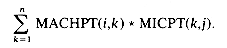
Observe that the number of MICPT(j) making up MACH(i) is
MACHPT(i,1) * MICPT(1,j) + MACHPT(i,2) * MICPT(2,j)
+ ... + MACHPT(i,n) * MICPT(n,j)
where the arrays are named MACHPT(m,n) and MICPT(n,p). This sum is more conveniently written as
If we compute these sums for each machine and each micropart then we will have a total of mp values which we might store in a third table MACHSUM(m,p). Regarding these tables as matrices this application leads to the general definition of matrix product:
Given A and B where A is m
for
Consider an algorithm which computes the product of two sparse matrices represented as an ordered list instead of an array. To compute the elements of C row-wise so we can store them in their proper place without moving previously computed elements, we must do the following: fix a row of A and find all elements in column j of B for j = 1,2,...,p. Normally, to find all the elements in column j of B we would have to scan all of B. To avoid this, we can first compute the transpose of B which will put all column elements consecutively. Once the elements in row i of A and column j of B have been located, we just do a merge operation similar to the polynomial addition of section 2.2. An alternative approach is explored in the exercises.
Before we write a matrix multiplication procedure, it will be useful to define a sub-procedure:
The algorithm MMULT which multiplies the matrices A and B to obtain the product matrix C uses the strategy outlined above. It makes use of variables i,j,q,r,col and row__begin. The variable r is the row of A that is currently being multiplied with the columns of B. row__begin is the position in A of the first element of row r. col is the column of B that is currently being multiplied with row r of A. q is the position in C for the next element generated. i and j are used to successively examine elements of row r and column col of A and B respectively. In addition to all this, line 6 of the algorithm introduces a dummy term into each of A and
We leave the correctness proof of this algorithm as an exercise. Let us examine its complexity. In addition to the space needed for A, B, C and some simple variables, space is also needed for the transpose matrix
When this happens, i is reset to row__begin in line 13. At the same time col is advanced to the next column. Hence, this resetting can take place at most p times (there are only p columns in B). The total maximum increments in i is therefore pdr. The maximum number of iterations of the while loop of lines 9-29 is therefore p + pdr + t2. The time for this loop while multiplying with row r of A is O(pdr + t2). Lines 30-33 take only O(dr) time. Hence, the time for the outer while loop, lines 7-34, for the iteration with row r of A is O(pdr + t2). The overall time for this loop is then O(
Once again, we may compare this computing time with the time to multiply matrices when arrays are used. The classical multiplication algorithm is:
The time for this is O(mnp). Since t1
The above analysis for MMULT is nontrivial. It introduces some new concepts in algorithm analysis and you should make sure you understand the analysis.
As in the case of polynomials, this representation for sparse matrices permits one to perform operations such as addition, transpose and multiplication efficiently. There are, however, other considerations which make this representation undesirable in certain applications. Since the number of terms in a sparse matrix is variable, we would like to represent all our sparse matrices in one array rather than using a separate array for each matrix. This would enable us to make efficient utilization of space. However, when this is done, we run into difficulties in allocating space from this array to any individual matrix. These difficulties also arise with the polynomial representation of the previous section and will become apparent when we study a similar representation for multiple stacks and queues (section 3.4).
Even though multidimensional arrays are provided as a standard data object in most high level languages, it is interesting to see how they are represented in memory. Recall that memory may be regarded as one dimensional with words numbered from 1 to m. So, we are concerned with representing n dimensional arrays in a one dimensional memory. While many representations might seem plausible, we must select one in which the location in memory of an arbitrary array element, say A(i1,i2, ...,in), can be determined efficiently. This is necessary since programs using arrays may, in general, use array elements in a random order. In addition to being able to retrieve array elements easily, it is also necessary to be able to determine the amount of memory space to be reserved for a particular array. Assuming that each array element requires only one word of memory, the number of words needed is the number of elements in the array. If an array is declared A(l1 :u1,l2:u2, ...,ln:un), then it is easy to see that the number of elements is
One of the common ways to represent an array is in row major order. If we have the declaration
A(4:5, 2:4, 1:2, 3:4)
then we have a total of 2
A(4,2,1,3), A(4,2,1,4), A(4,2,2,3), A(4,2,2,4)
and continuing
A(4,3,1,3), A(4,3,1,4), A(4,3,2,3), A(4,3,2,4)
for 3 more sets of four until we get
A(5,4,1,3), A(5,4,1,4), A(5,4,2,3), A(5,4,2,4).
We see that the subscript at the right moves the fastest. In fact, if we view the subscripts as numbers, we see that they are, in some sense, increasing:
4213,4214, ...,5423,5424.
Another synonym for row major order is lexicographic order.
From the compiler's point of view, the problem is how to translate from the name A(i1,i2, ...,in) to the correct location in memory. Suppose A(4,2,1,3) is stored at location 100. Then A(4,2,1,4) will be at 101 and A(5,4,2,4) at location 123. These two addresses are easy to guess. In general, we can derive a formula for the address of any element. This formula makes use of only the starting address of the array plus the declared dimensions.
To simplify the discussion we shall assume that the lower bounds on each dimension li are 1. The general case when li can be any integer is discussed in the exercises. Before obtaining a formula for the case of an n-dimensional array, let us look at the row major representation of 1, 2 and 3 dimensional arrays. To begin with, if A is declared A(1:u1), then assuming one word per element, it may be represented in sequential memory as in figure 2.3. If
The two dimensional array A(1:u1,1:u2) may be interpreted as u1 rows: row 1,row 2, ...,row u1, each row consisting of u2 elements. In a row major representation, these rows would be represented in memory as in figure 2.4.
Again, if
Figure 2.5 shows the representation of the 3 dimensional array A(1:u1,1:u2,1:u3). This array is interpreted as u1 2 dimensional arrays of dimension u2 x u3 . To locate A(i,j,k), we first obtain
Generalizing on the preceding discussion, the addressing formula for any element A(i1,i2, ...,in) in an n-dimensional array declared as A(u1,u2, ...,un) may be easily obtained. If
Repeating in this way the address for A(i1,i2, ...,in) is
Note that aj may be computed from
An alternative scheme for array representation, column major order, is considered in exercise 21.
To review, in this chapter we have used arrays to represent ordered lists of polynomials and sparse matrices. In all cases we have been able to move the values around, accessing arbitrary elements in a fixed amount of time, and this has given us efficient algorithms. However several problems have been raised. By using a sequential mapping which associates ai of (a1, ...,an) with the i-th element of the array, we are forced to move data around whenever an insert or delete operation is used. Secondly, once we adopt one ordering of the data we sacrifice the ability to have a second ordering simultaneously.
1. Write a SPARKS procedure which multiplies two polynomials represented using scheme 2 in Section 2.2. What is the computing time of your procedure?
2. Write a SPARKS procedure which evaluates a polynomial at a value x0 using scheme 2 as above. Try to minimize the number of operations.
3. If A = (a1, ...,an) and B = (b1, ...,bm) are ordered lists, then A < B if ai = bi for
4. Assume that n lists, n > 1, are being represented sequentially in the one dimensional array SPACE (1:m). Let FRONT(i) be one less than the position of the first element in the ith list and let REAR(i) point to the last element of the ith list, 1
a) Obtain suitable initial and boundary conditions for FRONT(i) and REAR(i)
b) Write a procedure INSERT(i,j,item) to insert item after the (j - 1)st element in list i. This procedure should fail to make an insertion only if there are already m elements in SPACE.
5. Using the assumptions of (4) above write a procedure DELETE(i,j,item) which sets item to the j-th element of the i-th list and removes it. The i-th list should be maintained as sequentially stored.
6. How much space is actually needed to hold the Fibonacci polynomials F0,F1, ..,F100?
7. In procedure MAIN why is the second dimension of F = 203?
8. The polynomials A(x) = x2n + x2n-2 + ... + x2 + x0 and B(x) = x2n+1 + x2n-l + ... + x3 + x cause PADD to work very hard. For these polynomials determine the exact number of times each statement will be executed.
9. Analyze carefully the computing time and storage requirements of algorithm FAST--TRANSPOSE. What can you say about the existence of an even faster algorithm?
10. Using the idea in FAST--TRANSPOSE of m row pointers, rewrite algorithm MMUL to multiply two sparse matrices A and B represented as in section 2.3 without transposing B. What is the computing time of your algorithm?
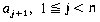
11. When all the elements either above or below the main diagonal of a square matrix are zero, then the matrix is said to be triangular. Figure 2.6 shows a lower and upper triangular matrix.
In a lower triangular matrix, A, with n rows, the maximum number of nonzero terms in row i is i. Hence, the total number of nonzero terms is
What is the relationship between i and j for elements in the zero part of A?
12. Let A and B be two lower triangular matrices, each with n rows. The total number of elements in the lower triangles is n(n + 1). Devise a scheme to represent both the triangles in an array C(1:n,1:n + 1). [Hint: represent the triangle of A as the lower triangle of C and the transpose of B as the upper triangle of C.] Write algorithms to determine the values of A(i,j), B(i,j) 1
13. Another kind of sparse matrix that arises often in numerical analysis is the tridiagonal matrix. In this square matrix, all elements other than those on the major diagonal and on the diagonals immediately above and below this one are zero
If the elements in the band formed by these three diagonals are represented rowwise in an array, B, with A (1,1) being stored at B(1), obtain an algorithm to determine the value of A(i,j), 1
14. Define a square band matrix An,a to be a n x n matrix in which all the nonzero terms lie in a band centered around the main diagonal. The band includes a - 1 diagonals below and above the main diagonal and also the main diagonal.
a) How many elements are there in the band of An,a?
b) What is the relationship between i and j for elements aij in the band of An,a?
c) Assume that the band of An,a is stored sequentially in an array B by diagonals starting with the lowermost diagonal. Thus A4,3 above would have the following representation:
Obtain an addressing formula for the location of an element aij in the lower band of An,a.
e.g. LOC(a31) = 1, LOC(a42) = 2 in the example above.
15. A generalized band matrix An,a,b is a n x n matrix A in which all the nonzero terms lie in a band made up of a - 1 diagonals below the main diagonal, the main diagonal and b - 1 diagonals above the main diagonal (see the figure on the next page)
a) How many elements are there in the band of An,a,b?
b) What is the relationship between i and j for elements aij in the band of An,a,b?
c) Obtain a sequential representation of the band of An,a,b in the one dimensional array B. For this representation write an algorithm VALUE (n,a,b,i,j,B) which determines the value of element aij in the matrix An,a,b. The band of An,a,b is represented in the array B.
16. How much time does it take to locate an arbitrary element A(i,j) in the representation of section 2.3 and to change its value?
17. A variation of the scheme discussed in section 2.3 for sparse matrix representation involves representing only the non zero terms in a one dimensional array VA in the order described. In addition, a strip of n x m bits, BA (n,m), is also kept. BA(i,j) = 0 if A(i,j) = 0 and BA(i,j) = 1 if A(i,j)
(i) On a computer with w bits per word, how much storage is needed to represent a sparse matrix Anxm with t nonzero terms?
(ii) Write an algorithm to add two sparse matrices A and C represented as above to obtain D = A + C. How much time does your algorithm take ?
(iii) Discuss the merits of this representation versus the representation of section 2.3. Consider space and time requirements for such operations as random access, add, multiply, and transpose. Note that the random access time can be improved somewhat by keeping another array RA(i) such that RA(i) = number of nonzero terms in rows 1 through i - 1.
18. A complex-valued matrix X is represented by a pair of matrices (A,B) where A and B contain real values. Write a program which computes the product of two complex valued matrices (A,B) and (C,D), where
(A,B) * (C,D) = (A + iB) * (C + iD) = (AC - BD) + i(AD + BC)
Determine the number of additions and multiplications if the matrices are all n
19. How many values can be held by an array with dimensions A(0:n), B(-1:n,1:m), C(-n:0,2)?
20. Obtain an addressing formula for the element A(i1,i2, ...,in) in an array declared as A(l1:ul,l2:u2, ...,ln:un). Assume a row major representation of the array with one word per element and
21. Do exercise 20 assuming a column major representation. In this representation, a 2 dimensional array is stored sequentially by column rather than by rows.
22. An m X n matrix is said to have a saddle point if some entry A(i,j) is the smallest value in row i and the largest value in column j. Write a SPARKS program which determines the location of a saddle point if one exists. What is the computing time of your method?
23. Given an array A(1:n) produce the array Z(1:n) such that Z(1) = A(n), Z(2) = A(n - 1), ..., Z(n - 1) = A(2), Z(n) = A(1). Use a minimal amount of storage.
24. One possible set of axioms for an ordered list comes from the six operations of section 2.2.
Use these axioms to describe the list A = (a, b, c, d, e) and show what happens when DEL (A,2) is executed.
25. There are a number of problems, known collectively as "random walk" problems which have been of long standing interest to the mathematical community. All but the most simple of these are extremely difficult to solve and for the most part they remain largely unsolved. One such problem may be stated as follows:
A (drunken) cockroach is placed on a given square in the middle of a tile floor in a rectangular room of size n x m tiles. The bug wanders (possibly in search of an aspirin) randomly from tile to tile throughout the room. Assuming that he may move from his present tile to any of the eight tiles surrounding him (unless he is against a wall) with equal probability, how long will it take him to touch every tile on the floor at least once?
Hard as this problem may be to solve by pure probability theory techniques, the answer is quite easy to solve using the computer. The technique for doing so is called "simulation" and is of wide-scale use in industry to predict traffic-flow, inventory control and so forth. The problem may be simulated using the following method:
An array K
A random walk to one of the 8 given squares is simulated by generating a random value for K lying between 1 and 8. Of course the bug cannot move outside the room, so that coordinates which lead up a wall must be ignored and a new random combination formed. Each time a square is entered, the count for that square is incremented so that a non-zero entry shows the number of times the bug has landed on that square so far. When every square has been entered at least once, the experiment is complete.
Write a program to perform the specified simulation experiment. Your program MUST:
1) Handle values of N and M
2 < N
2
2) Perform the experiment for
a) N = 15, M = 15 starting point: (20,10)
b) N = 39, M = 19 starting point: (1,1)
3) Have an iteration limit, that is, a maximum number of squares the bug may enter during the experiment. This assures that your program does not get "hung" in an "infinite" loop. A maximum of 50,000 is appropriate for this lab.
4) For each experiment print: a) the total number of legal moves which the cockroach makes; b) the final K
(Have an aspirin) This exercise was contributed by Olson.
26. Chess provides the setting for many fascinating diversions which are quite independent of the game itself. Many of these are based on the strange "L-shaped" move of the knight. A classical example is the problem of the knight's tour, which has captured the attention of mathematicians and puzzle enthusiasts since the beginning of the eighteenth century. Briefly stated, the problem is to move the knight, beginning from any given square on the chessboard, in such a manner that it travels successively to all 64 squares, touching each square once and only once. It is convenient to represent a solution by placing the numbers 1,2, ...,64 in the squares of the chessboard indicating the order in which the squares are reached. Note that it is not required that the knight be able to reach the initial position by one more move; if this is possible the knight's tour is called re-entrant.
One of the more ingenious methods for solving the problem of the knight's tour is that given by J. C. Warnsdorff in 1823. His rule is that the knight must always be moved to one of the squares from which there are the fewest exits to squares not already traversed.
The goal of this exercise is to write a computer program to implement Warnsdorff's rule. The ensuing discussion will be much easier to follow, however, if the student will first try to construct a particular solution to the problem by hand before reading any further.
The most important decisions to be made in solving a problem of this type are those concerning how the data is to be represented in the computer. Perhaps the most natural way to represent the chessboard is by an 8 x 8 array B
In general a knight at (I,J) may move to one of the squares (I - 2,J + 1), (I -1,J + 2), (I + 1,J + 2), (I + 2,J + 1), (I + 2,J - 1), (I + 1,J - 2), (I -1,J - 2), (I - 2,J - 1). Notice, however that if (I,J) is located near one of the edges of the board, some of these possibilities could move the knight off the board, and of course this is not permitted. The eight possible knight moves may conveniently be represented by two arrays KTM
Then a knight at (I,J) may move to (I + KTM
Below is a description of an algorithm for solving the knight's tour problem using Warnsdorff's rule. The data representation discussed in the previous section is assumed.
a. [Initialize chessboard] For 1
b. [Set starting position] Read and print I,J and then set B
c. [Loop] For 2
d. [Form set of possible next squares] Test each of the eight squares one knight's move away from (I,J) and form a list of the possibilities for the next square (NEXTI(L), NEXTJ(L)). Let NP
e. [Test special cases] If NP
f. [Find next square with minimum number of exits] For 1
g. [Move knight] Set I = NEXTI(MIN), J = NEXTJ(MIN) and B
h. [Print] Print out B
The problem is to write a program which corresponds to this algorithm. This exercise was contributed by Legenhausen and Rebman.
structure ARRAY(value, index)
declare CREATE( )
 array
arrayRETRIEVE(array,index)
valueSTORE(array,index,value)
array;for all A
 array, i,j index, x value let
RETRIEVE(CREATE,i) :: = error
RETRIEVE(STORE(A,i,x),j) :: =
if EQUAL(i,j) then x else RETRIEVE(A,j)
end
end ARRAY
2.2 ORDERED LISTS
 ;
; ;
; causing elements numbered i,i + 1, ...,n to become numbered i + 1,i + 2, ...,n + 1;
 causing elements numbered i + 1, ...,n to become numbered i,i + 1, ...,n - 1.
structure POLYNOMIAL
declare ZERO( )
poly; ISZERO(poly) BooleanCOEF(poly,exp)
coef;ATTACH(poly,coef,exp)
polyREM(poly,exp)
polySMULT(poly,coef,exp)
polyADD(poly,poly)
poly; MULT(poly,poly) poly;for all P,Q,
poly c,d, coef e,f exp letREM(ZERO,f) :: = ZERO
REM(ATTACH(P,c,e),f) :: =
if e = f then REM(P,f) else ATTACH(REM(P,f),c,e)
ISZERO(ZERO) :: = true
ISZERO(ATTACH(P,c,e)):: =
if COEF(P,e) = - c then ISZERO(REM(P,e)) else false
COEF(ZERO,e) :: = 0
COEF(ATTACH(P,c,e),f) :: =
if e = f then c + COEF(P,f) else COEF(P,f)
SMULT(ZERO,d,f) :: = ZERO
SMULT(ATTACH(P,c,e),d,f) :: =
ATTACH(SMULT(P,d,f),c
 d,e + f)
ADD(P,ZERO):: = P
ADD(P,ATTACH(Q,d,f)) :: = ATTACH(ADD(P,Q),d,f)
MULT(P,ZERO) :: = ZERO
MULT(P,ATTACH(Q,d,f)) :: =
ADD(MULT(P,Q),SMULT(P,d,f))
end
end POLYNOMIAL
exp which returns the leading exponent of poly, we can write a version of ADD which is expressed more like program, but is still representation independent.//C = A + B where A,B are the input polynomials//
C
 ZERO
ZEROwhile not ISZERO(A) and not ISZERO(B) do
case
: EXP(A) < EXP(B):
C
ATTACH(C,COEF(B,EXP(B)),EXP(B))B
REM(B,EXP(B)):EXP(A) = EXP(B):
C
ATTACH(C,COEF(A,EXP(A))+COEF(B,EXP(B)),EXP(A))A
REM(A,EXP(A)); B REM(B,EXP(B)):EXP(A) > EXP(B):
C
ATTACH(C,COEF(A,EXP(A)),EXP(A))A
REM(A,EXP(A))end
end
 0 and we say that the degree of A is n. Then we can represent A(x) as an ordered list of coefficients using a one dimensional array of length n + 2,
(1)
 . If all of A's coefficients are nonzero, then m = n + 1, ei = i, and bi = ai for
  . Alternatively, only an may be nonzero, in which case m = 1, bo = an, and e0 = n. In general, the polynomial in (1) could be represented by the ordered list of length 2m + 1,
procedure PADD(A,B,C)
//A(1:2m + 1), B(1:2n + 1), C(1:2(m + n) + 1)//
1 m
A(1); n B(l)2 p
q r 23 while p
 2m and q 2n do
4 case //compare exponents//
:A(p) = B(q): C(r + 1)
A(p + 1) + B(q + 1)//add coefficients//
if C(r + 1)
0then [C(r)
A(p); r r + 2]//store exponent//
p
p + 2; q q + 2 //advance to nextterms//
:A(p) < B(q): C(r + 1)
B(q + 1); C(r) B(q)//store new term//
q
q + 2; r r + 2 //advance to nextterm//
:A(p) > B(q): C(r + 1)
A(p + 1); C(r) A(p)//store new term//
p
p + 2; r r + 2 //advance to nextterm//
end
end
5 while p
 2m do //copy remaining terms of A//
C(r)
A(p); C(r + 1) A(p + 1)p
p + 2 ; r r + 2end
6 while q
 2n do //copy remaining terms of B//
C(r)
B(q); C(r + 1) B(q + 1)q
q + 2; r r + 2end
7 C(l)
r/2 - 1 //number of terms in the sum//end PADD
2; q r; p q ni=0x2i and B(x) = ni=0x2i+1 Since none of the exponents are the same in A and B, A(p) B(q). Consequently, on each iteration the value of only one of p or q increases by 2. So, the worst case computing time for this while loop is O(n + m). The total computing time for the while loops of lines 5 and 6 is bounded by O(n + m), as the first cannot be iterated more than m times and the second more than n . Taking the sum of all of these steps, we obtain O(n + m) as the asymptotic computing time of this algorithm.
 Fl (x) + F0(x) = x2 + 1.
procedure MAIN
declare F(0:100,203),TEMP(203)
read (n)
if n > 100 then [print ('n too large') stop]F(0,*)
(1,0,1) //set Fo = 1x0//F(1,*)
(1,1,1) //set F1 = 1x1//for i
2 to n docall PMUL(F(1,1),F(i - 1,1),TEMP(1)) //TEMP=x
Fi-(x)//
call PADD(TEMP(1),F(i - 2,1),F(i,1)) //Fi = TEMP +
Fi-2//
//TEMP is no longer needed//
end
for i
0 to n docall PPRINT(F(i,1)) //polynomial print routine//
end
end MAIN
 free and free free + 2k + 1. Now we have localized all storage to one array. As we create polynomials, free is continually incremented until it tries to exceed max. When this happens must we quit? We must unless there are some polynomials which are no longer needed. There may be several such polynomials whose space can be reused. We could write a subroutine which would compact the remaining polynomials, leaving a large, consecutive free space at one end. But this may require much data movement. Even worse, if we move a polynomial we must change its pointer. This demands a sophisticated compacting routine coupled with a disciplined use of names for polynomials. In Chapter 4 we will see an elegant solution to these problems.
2.3 SPARSE MATRICES
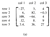

Figure 2.1: Example of 2 matrices
1, 2, 3
------------
A(0, 6, 6, 8
(1, 1, 1, 15
(2, 1, 4, 22
(3, 1, 6, -15
(4, 2, 2, 11
(5, 2, 3, 3
(6, 3, 4, -6
(7, 5, 1, 91
(8, 6, 3, 28
Figure 2.2: Sparse matrix stored as triples
1, 2, 3
--------------
B(0, 6, 6, 8
(1, 1, 1, 15
(2, 1, 5, 91
(3, 2, 2, 11
(4, 3, 2, 3
(5, 3, 6, 28
(6, 4, 1, 22
(7, 4, 3, -6
(8, 6, 1, -15
for each row i do
take element (i,j,val) and
store it in (j,i,val) of the transpose
end
for all elements in column j do
place element (i,j,val) in position (j,i,val)
end
procedure TRANSPOSE (A,B)
// A is a matrix represented in sparse form//
// B is set to be its transpose//
1 (m,n,t)
(A(0,l),A(0,2),A(0,3))2 (B(0,1),B(0,2),B(0,3))
(n,m,t)3 if t
 0 then return //check for zero matrix//
4 q
1 //q is position of next term in B//5 for col
1 to n do //transpose by columns//6 for p
1 to t do //for all nonzero terms do//7 if A(p,2) = col //correct column//
8 then [(B(q,1),B(q,2),B(q,3))
//insert next termof B//
9 (A(p,2),A(p,1),A(p,3))
10 q
q + 1]11 end
12 end
13 end TRANSPOSE
(d,e,f) d; b e; c f.for j
1 to n dofor i
1 to m doB(j,i)
A(i,j)end
end
procedure FAST--TRANSPOSE(A,B)
//A is an array representing a sparse m X n matrix with t nonzero
terms. The transpose is stored in B using only O(t + n)
operations//
declare S(1:n),T(1:n); //local arrays used as pointers//
1 (m,n,t)
(A(0,1),A(0,2),A(0,3))2 (B(0,1),B(0,2),B(0,3))
(n,m,t) //store dimensions oftranspose//
3 if t
 0 then return //zero matrix//
4 for i
1 to n do S(i) 0 end5 for i
1 to t do //S(k) is the number of//6 S(A(i,2))
S(A(i,2)) + 1 //elements in row k of B//7 end
8 T(1)
19 for i
2 to n do //T(i) is the starting//10 T(i)
T(i - 1) + S(i - 1) //position of row i inB//
11 end
12 for i
1 to t do //move all t elements of A to B//13 j
A(i,2) //j is the row in B//14 (B(T(j),1),B(T(j),2),B(T(j),3))
//store in triple//15 (A(i,2),A(i,1),A(i,3))
16 T(j)
T(j) + 1 //increase row j to next spot//17 end
18 end FAST--TRANSPOSE
(1) (2) (3) (4) (5) (6)
S = 2 1 2 2 0 1
T = 1 3 4 6 8 8
PART(1) PART(2) PART(3) ... PART(n)
----------------------------------------
MACH(1) | 0, 5, 2, ..., 0
MACH(2) | 0, 0, 0, ..., 3
MACH(3) | 1, 1, 0, ..., 8
. | . . . .
. | . . . .
. | . . . .
MACH(m) | 6, 0, 0, ..., 7
|
| array MACHPT(m,n)
 n and B is n p, the product matrix C has dimension m p. Its i,j element is defined as
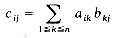
 and
and  . The product of two sparse matrices may no longer be sparse, for instance,
procedure STORESUM (C,q,row,col,sum)
//if sum is nonzero then along with its row and column position
it is stored into the q-th entry of the matrix//
if sum
0 then [(C(q,1),C(q,2),C(q,3) (row,col,sum)
q
q + 1; sum 0]end STORESUM
 . This enables us to handle end conditions (i.e., computations involving the last row of A or last column of B) in an elegant way.
 . Algorithm FAST__TRANSPOSE also needs some additional space. The exercises explore a strategy for MMULT which does not explicitly compute
  and the only additional space needed is the same as that required by FAST__TRANSPOSE. Turning our attention to the computing time of MMULT, we see that lines 1-6 require only O(p + t2) time. The while loop of lines 7-34 is executed at most m times (once for each row of A). In each iteration of the while loop of lines 9-29 either the value of i or j or of both increases by 1 or i and col are reset. The maximum total increment in j over the whole loop is t2. If dr is the number of terms in row r of A then the value of i can increase at most dr times before i moves to the next row of A.
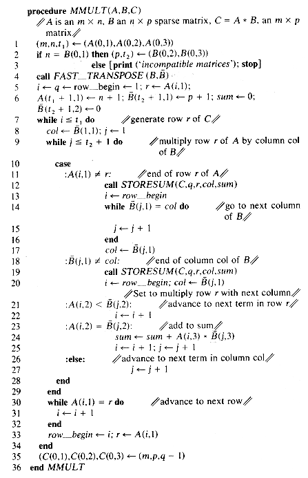 r(pdr + t2)) = O(pt1 + mt2).
for i
1 to m dofor j
1 to p dosum
0for k
1 to n dosum
sum + A(i,k) * B(k,j)end
C(i,j)
sumend
end
nm and t2 np, the time for MMULT is at most O(mnp). However, its constant factor is greater than that for matrix multiplication using arrays. In the worst case when t1 = nm or t2 = np, MMULT will be slower by a constant factor. However, when t1 and t2 are sufficiently smaller than their maximum values i.e., A and B are sparse, MMULT will outperform the above multiplication algorithm for arrays.2.4 REPRESENTATION OF ARRAYS
 3 2 2 = 24 elements. Then using row major order these elements will be stored as
 is the address of A(1), then the address of an arbitrary element A(i) is just + (i - 1).
array element: A(l), A(2), A(3), ..., A(i), ..., A(u1)
address:
, + 1, + 2, ..., + i - 1, ..., + u1 - 1 total number of elements = u1
Figure 2.3: Sequential representation of A(1:u1)
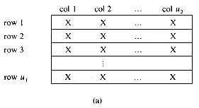

Figure 2.4: Sequential representation of A(u1,u2)
is the address of A(1 ,1), then the address of A(i,1) is + (i - 1)u2, as there are i - 1 rows each of size u2 preceding the first element in the i-th row. Knowing the address of A(i,1), we can say that the address of A(i,j) is then simply + (i - 1)u2 + (j - 1). + (i - 1) u2 u3 as the address for A(i,1,1) since there are i- 1 2 dimensional arrays of size u2 x u3 preceding this element. From this and the formula for addressing a 2 dimensional array, we obtain + (i - 1) u2 u3 + (j - 1) u3 + (k - 1) as the address of A(i,j,k). is the address for A(1,1, ...,1) then + (i1, - 1)u2u3 ... un is the address for A(i1,l, ...,1). The address for A(i1,i2,1, ...,1) is then + (i1, - 1)u2u3 ... un + (i2 - 1)u3u4 ... un.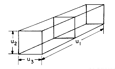
(a) 3-dimensional array A(u1,u2,u3) regarded as u1 2-dimensional arrays.
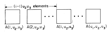
(b) Sequential row major representation of a 3-dimensional array. Each 2-dimensional array is represented as in Figure 2.4.
Figure 2.5: Sequential representation of A(u1,u2,u3)
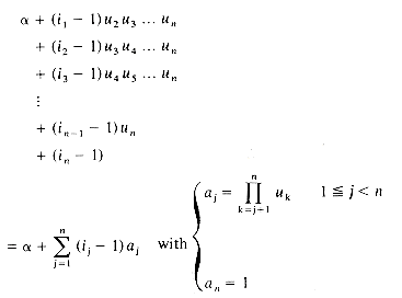
 using only one multiplication as aj = uj+1 aj+1. Thus, a compiler will initially take the declared bounds u1, ...,un and use them to compute the constants a1, ...,an-1 using n - 2 multiplications. The address of A(i1, ...,in) can then be found using the formula, requiring n - 1 more multiplications and n additions.
EXERCISES
 and aj < bj or if ai = bi for
  and n < m. Write a procedure which returns -1,0, + 1 depending upon whether A < B, A = B or A > B. Assume you can compare atoms ai and bj. i n. Further assume that REAR(i) FRONT(i + 1), 1 i n with FRONT(n + 1) = m. The functions to be performed on these lists are insertion and deletion.
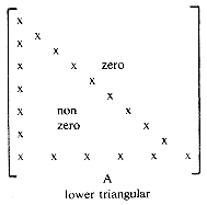
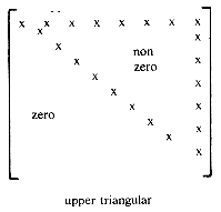
Figure 2.6
ni=1 i = n(n + 1)/2. For large n it would be worthwhile to save the space taken by the zero entries in the upper triangle. Obtain an addressing formula for elements aij in the lower triangle if this lower triangle is stored by rows in an array B(1:n(n + 1)/2) with A(1,1) being stored in B(1). i, j n from the array C.
Figure 2.7: Tridiagonal matrix A
i, j n from the array B.
B(1) B(2) B(3) B(4) B(5) B(6) B(7) B(8) B(9) B(10) B(11) B(12) B(13) B(14)
9 7 8 3 6 6 0 2 8 7 4 9 8 4
a31 a42 a21 a32 a43 a11 a22 a33 a44 a12 a23 a34 a13 a24
 0. The figure below illustrates the representation for the sparse matrix of figure 2.1.
 n. the address of A(l1,l2, ...,ln).
structure ORDERED__LlST(atoms)
declare MTLST( )
listLEN(list)
integerRET(list,integer)
atomSTO(list,integer,atom)
listINS(list,integer,atom)
listDEL(list,integer)
list;for all L
list, i.j integer a,b atom letLEN(MTLST) :: = 0; LEN(STO(L,i,a)) :: = 1 + LEN(L)
RET(MTLST,j) :: = error
RET(STO(L,i,a),j) :: =
if i = j then a else RET(L,j)
INS(MTLST,j,b) :: = STO(MTLST,j,b)
INS(STO(L,i,a),j,b) :: =
if i
 j then STO(INS(L,j,b), i + 1,a)
else STO(INS(L,j,b),i,a)
DEL(MTLST,j) :: = MTLST
DEL(STO(L,i,a),j) :: =
if i = j then DEL(L,j)
else if i > j then STO(DEL(L,j),i - 1,a)
else STO(DEL(L,j),i,a)
end
end ORDERED__LIST
 UNT dimensioned N X M is used to represent the number of times our cockroach has reached each tile on the floor. All the cells of this array are initialized to zero. The position of the bug on the floor is represented by the coordinates (IBUG,JBUG) and is initialized by a data card. The 8 possible moves of the bug are represented by the tiles located at (IBUG + IMVE(K), JBUG + JMVE(K)) where 1 K 8 and:
IM
VE(1) = -1 JMVE(1) = 1IM
VE(2) = 0 JMVE(2) = 1IM
VE(3) = 1 JMVE(3) = 1IM
VE(4) = 1 JMVE(4) = 0IM
VE(5) = 1 JMVE(5) = -1IM
VE(6) = 0 JMVE(6) = -1IM
VE(7) = -1 JMVE(7) = -1IM
VE(8) = -1 JMVE(8) = 0 40 M 20UNT array. This will show the "density" of the walk, that is the number of times each tile on the floor was touched during the experiment.ARD as shown in the figure below. The eight possible moves of a knight on square (5,3) are also shown in the figure.B
ARD 1 2 3 4 5 6 7 8
----------------------
1
2
3 8 1
4 7 2
5 K
6 6 3
7 5 4
8
V1 and KTMV2 as shown below.KTM
V1 KTMV2 -2 1
-1 2
1 2
2 1
2 -1
1 -2
-1 -2
-2 -1
V1(K), J + KTMV2(K)), where K is some value between 1 and 8, provided that the new square lies on the chessboard. I,J 8 set BARD(I,J) = 0.ARD(I,J) to 1. M 64 do steps d through g.S be the number of possibilities. (That is, after performing this step we will have NEXTI(L) = I + KTMV1(K) and NEXTJ(L) = J + KTMV2(K), for certain values of K between 1 and 8. Some of the squares (I + KTMV1(K), J + KTMV2(K)) may be impossible for the next move either because they lie off the chessboard or because they have been previously occupied by the knight--i.e., they contain a nonzero number. In every case we will have 0 NPS 8.)S = 0 the knight's tour has come to a premature end; report failure and then go to step h. If NPS = 1 there is only one possibility for the next move; set MIN = 1 and go right to step g. L NPS set EXITS(L) to the number of exits from square (NEXTI(L),NEXTJ(L)). That is, for each of the values of L examine each of the next squares (NEXTI(L) + KTMV1(K), NEXTJ(L) + KTMV2(K)) to see if it is an exit from NEXTI(L), NEXTJ(L)), and count the number of such exits in EXITS(L). (Recall that a square is an exit if it lies on the chessboard and has not been previously occupied by the knight.) Finally, set MIN to the location of the minimum value of EXITS. (There may be more than one occurrences of the minimum value of EXITS. If this happens, it is convenient to let MIN denote the first such occurrence, although it is important to realize that by so doing we are not actually guaranteed of finding a solution. Nevertheless, the chances of finding a complete knight's tour in this way are remarkably good, and that is sufficient for the purposes of this exercise.)ARD(I,J) = M. (Thus, (I,J) denotes the new position of the knight, and BARD(I,J) records the move in proper sequence.)ARD showing the solution to the knight's tour, and then terminate the algorithm.