


In this chapter we consider techniques to sort large files. The files are assumed to be so large that the whole file cannot be contained in the internal memory of a computer, making an internal sort impossible. Before discussing methods available for external sorting it is necessary first to study the characteristics of the external storage devices which can be used to accomplish the sort. External storage devices may broadly be categorized as either sequential access (e.g., tapes) or direct access (e.g., drums and disks). Section 8.1 presents a brief study of the properties of these devices. In sections 8.2 and 8.3 we study sorting methods which make the best use of these external devices.
Magnetic tape devices for computer input/output are similar in principle to audio tape recorders. The data is recorded on magnetic tape approximately 1/2\" wide. The tape is wound around a spool. A new reel of tape is normally 2400 ft. long (with use, the length of tape in a reel tends to decrease because of frequent cutting off of lengths of the tape). Tracks run across the length of the tape, with a tape having typically 7 to 9 tracks across its width. Depending on the direction of magnetization, a spot on the track can represent either a 0 or a 1 (i.e., a bit of information). At any point along the length of the tape, the combination of bits on the tracks represents a character (e.g., A-Z, 0-9, +, :, ;, etc.). The number of bits that can be written per inch of track is referred to as the tape density. Examples of standard track densities are 800 and 1600 bpi (bits per inch). Since there are enough tracks across the width of the tape to represent a character, this density also gives the number of characters per inch of tape. Figure 8.1 illustrates this. With the conventions of the figure, the code for the first character on the tape is 10010111 while that for the third character is 00011100. If the tape is written using a density of 800 bpi then the length marked x in the figure is 3/800 inches.
Reading from a magnetic tape or writing onto one is done from a tape drive, as shown in figure 8.2. A tape drive consists of two spindles. On one of the spindles is mounted the source reel and on the other the take up reel. During forward reading or forward writing, the tape is pulled from the source reel across the read/write heads and onto the take up reel. Some tape drives also permit backward reading and writing of tapes; i.e., reading and writing can take place when tape is being moved from the take up to the source reel.
If characters are packed onto a tape at a density of 800 bpi, then a 2400 ft. tape would hold a little over 23 x 106 characters. A density of 1600 bpi would double this figure. However, it is necessary to block data on a tape since each read/write instruction transmits a whole block of information into/from memory. Since normally we would neither have enough space in memory for one full tape load nor would we wish to read the whole tape at once, the information on a tape will be grouped into several blocks. These blocks may be of a variable or fixed size. In between blocks of data is an interblock gap normally about 3/4 inches long. The interblock gap is long enough to permit the tape to accelerate from rest to the correct read/write speed before the beginning of the next block reaches the read/write heads. Figure 8.3 shows a segment of tape with blocked data.
In order to read a block from a tape one specifies the length of the block and also the address, A, in memory where the block is to be transmitted. The block of data is packed into the words A, A + 1, A + 2, .... Similarly, in order to write a block of data onto tape one specifies the starting address in memory and the number of consecutive words to be written. These input and output areas in memory will be referred to as buffers. Usually the block size will correspond to the size of the input/output buffers set up in memory. We would like these blocks to be as large as possible for the following reasons:
(i) Between any pair of blocks there is an interblock gap of 3/4\". With a track density of 800 bpi, this space is long enough to write 600 characters. Using a block length of 1 character/block on a 2400 ft. tape would result in roughly 38,336 blocks or a total of 38,336 characters on the entire tape. Tape utilization is 1/601 < 0.17%. With 600 characters per block, half the tape would be made up of interblock gaps. In this case, the tape would have only about 11.5 x 10⁶ characters of information on it, representing a 50% utilization of tape. Thus, the longer the blocks the more characters we can write onto the tape.
(ii) If the tape starts from rest when the input/output command is issued, then the time required to write a block of n characters onto the tape is ta + ntw where ta is the delay time and tw the time to transmit one character from memory to tape. The delay time is the time needed to cross the interblock gap. If the tape starts from rest then ta includes the time to accelerate to the correct tape speed. In this case ta is larger than when the tape is already moving at the correct speed when a read/write command is issued. Assuming a tape speed of 150 inches per second during read/write and 800 bpi the time to read or write a character is 8.3 x 10⁻⁶sec. The transmission rate is therefore 12 x 104 characters/second. The delay time ta may typically be about 10 milliseconds. If the entire tape consisted of just one long block, then it could be read in
While large blocks are desirable from the standpoint of efficient tape usage as well as reduced input/output time, the amount of internal memory available for use as input/output buffers puts a limitation on block size.
Computer tape is the foremost example of a sequential access device. If the read head is positioned at the front of the tape and one wishes to read the information in a block 2000 ft. down the tape then it is necessary to forward space the tape the correct number of blocks. If now we wish to read the first block, the tape would have to be rewound 2000 ft. to the front before the first block could be read. Typical rewind times over 2400 ft. of tape could be around one minute.
Unless otherwise stated we will make the following assumptions about our tape drives:
(i) Tapes can be written and read in the forward direction only.
(ii) The input/output channel of the computer is such as to permit the following three tasks to be carried out in parallel: writing onto one tape, reading from another and CPU operation.
(iii) If blocks 1, ...,i have been written on a tape, then the tape can be moved backwards block by block using a backspace command or moved to the first block via a rewind command. Overwriting block i- 1 with another block of the same size destroys the leading portion of block i. While this latter assumption is not true of all tape drives, it is characteristic of most of them.
As an example of direct access external storage, we consider disks. As in the case of tape storage, we have here two distinct components: (1) the disk module (or simply disk or disk pack) on which information is stored (this corresponds to a reel of tape in the case of tape storage) and (2) the disk drive (corresponding to the tape drive) which performs the function of reading and writing information onto disks. Like tapes, disks can be removed from or mounted onto a disk drive. A disk pack consists of several platters that are similar to phonograph records. The number of platters per pack varies and typically is about 6. Figure 8.4 shows a disk pack with 6 platters. Each platter has two surfaces on which information can be recorded. The outer surfaces of the top and bottom platters are not used. This gives the disk of figure 8.4 a total of 10 surfaces on which information may be recorded. A disk drive consists of a spindle on which a disk may be mounted and a set of read/write heads. There is one read/write head for each surface. During a read/write the heads are held stationary over the position of the platter where the read/write is to be performed, while the disk itself rotates at high speeds (speeds of 2000-3000 rpm are fairly common). Thus, this device will read/write in concentric circles on each surface. The area that can be read from or written onto by a single stationary head is referred to as a track. Tracks are thus concentric circles, and each time the disk completes a revolution an entire track passes a read/write head. There may be from 100 to 1000 tracks on each surface of a platter. The collection of tracks simultaneously under a read/write head on the surfaces of all the platters is called a cylinder. Tracks are divided into sectors. A sector is the smallest addressable segment of a track. Information is recorded along the tracks of a surface in blocks. In order to use a disk, one must specify the track or cylinder number, the sector number which is the start of the block and also the surface. The read/write head assembly is first positioned to the right cylinder. Before read/write can commence, one has to wait for the right sector to come beneath the read/write head. Once this has happened, data transmission can take place. Hence, there are three factors contributing to input/output time for disks:
(i) Seek time: time taken to position the read/write heads to the correct cylinder. This will depend on the number of cylinders across which the heads have to move.
(ii) Latency time: time until the right sector of the track is under the read/write head.
(iii) Transmission time: time to transmit the block of data to/from the disk.
Maximum seek times on a disk are around 1/10 sec. A typical revolution speed for disks is 2400 rpm. Hence the latency time is at most 1/40 sec (the time for one revolution of the disk). Transmission rates are typically between 105 characters/second and 5 x 10⁵ characters/second. The number of characters that can be written onto a disk depends on the number of surfaces and tracks per surface. This figure ranges from about 107 characters for small disks to about 5 x 10⁸ characters for a large disk.
The most popular method for sorting on external storage devices is merge sort. This method consists of essentially two distinct phases. First, segments of the input file are sorted using a good internal sort method. These sorted segments, known as runs, are written out onto external storage as they are generated. Second, the runs generated in phase one are merged together following the merge tree pattern of Example 7.4, until only one run is left. Because the merge algorithm of section 7.5 requires only the leading records of the two runs being merged to be present in memory at one time, it is possible to merge large runs together. It is more difficult to adapt the other methods considered in Chapter 7 to external sorting. Let us look at an example to illustrate the basic external merge sort process and analyze the various contributions to the overall computing time. A file containing 4500 records, A1, . . . ,A4500, is to be sorted using a computer with an internal memory capable of sorting at most 750 records. The input file is maintained on disk and has a block length of 250 records. We have available another disk which may be used as a scratch pad. The input disk is not to be written on. One way to accomplish the sort using the general procedure outlined above is to:
(i) Internally sort three blocks at a time (i.e., 750 records) to obtain six runs R1-R6. A method such as heapsort or quicksort could be used. These six runs are written out onto the scratch disk (figure 8.5).
(ii) Set aside three blocks of internal memory, each capable of holding 250 records. Two of these blocks will be used as input buffers and the third as an output buffer. Merge runs R1 and R2. This is carried out by first reading one block of each of these runs into input buffers. Blocks of runs are merged from the input buffers into the output buffer. When the output buffer gets full, it is written out onto disk. If an input buffer gets empty, it is refilled with another block from the same run. After runs R1 and R2 have been merged, R3 and R4 and finally R5 and R6 are merged. The result of this pass is 3 runs, each containing 1500 sorted records of 6 blocks. Two of these runs are now merged using the input/output buffers set up as above to obtain a run of size 3000. Finally, this run is merged with the remaining run of size 1500 to obtain the desired sorted file (figure 8.6).
Let us now analyze the method described above to see how much time is required to sort these 4500 records. The analysis will use the following notation:
ts = maximum seek time
tl = maximum latency time
trw = time to read or write one block of 250 records
tIO = ts + tl + trw
tIS = time to internally sort 750 records
n tm = time to merge n records from input buffers to the output buffer
We shall assume that each time a block is read from or written onto the disk, the maximum seek and latency times are experienced. While this is not true in general, it will simplify the analysis. The computing time for the various operations are:
Note that the contribution of seek time can be reduced by writing blocks on the same cylinder or on adjacent cylinders. A close look at the final computing time indicates that it depends chiefly on the number of passes made over the data. In addition to the initial input pass made over the data for the internal sort, the merging of the runs requires 2-2/3 passes over the data (one pass to merge 6 runs of length 750 records, two thirds of a pass to merge two runs of length 1500 and one pass to merge one run of length 3000 and one of length 1500). Since one full pass covers 18 blocks, the input and output time is 2 X (2-2/3 + 1) X 18 tIO = 132 tIO. The leading factor of 2 appears because each record that is read is also written out again. The merge time is 2-2/3 X 4500 tm = 12,000 tm. Because of this close relationship between the overall computing time and the number of passes made over the data, future analysis will be concerned mainly with counting the number of passes being made. Another point to note regarding the above sort is that no attempt was made to use the computer's ability to carry out input/output and CPU operation in parallel and thus overlap some of the time. In the ideal situation we would overlap almost all the input/output time with CPU processing so that the real time would be approximately 132 tIO
If we had two disks we could write on one while reading from the other and merging buffer loads already in memory all at the same time. In this case a proper choice of buffer lengths and buffer handling schemes would result in a time of almost 66 tIO. This parallelism is an important consideration when the sorting is being carried out in a non-multi-programming environment. In this situation unless input/output and CPU processing is going on in parallel, the CPU is idle during input/output. In a multi-programming environment, however, the need for the sorting program to carry out input/output and CPU processing in parallel may not be so critical since the CPU can be busy working on another program (if there are other programs in the system at that time), while the sort program waits for the completion of its input/output. Indeed, in many multi-programming environments it may not even be possible to achieve parallel input, output and internal computing because of the structure of the operating system.
The remainder of this section will concern itself with: (1) reduction of the number of passes being made over the data and (2) efficient utilization of program buffers so that input, output and CPU processing is overlapped as much as possible. We shall assume that runs have already been created from the input file using some internal sort scheme. Later, we investigate a method for obtaining runs that are on the average about 2 times as long as those obtainable by the methods discussed in Chapter 7.
The 2-way merge algorithm of Section 7.5 is almost identical to the merge procedure just described (figure 8.6). In general, if we started with m runs, then the merge tree corresponding to figure 8.6 would have
The construction of this selection tree may be compared to the playing of a tournament in which the winner is the record with the smaller key. Then, each nonleaf node in the tree represents the winner of a tournament and the root node represents the overall winner or the smallest key. A leaf node here represents the first record in the corresponding run. Since the records being sorted are generally large, each node will contain only a pointer to the record it represents. Thus, the root node contains a pointer to the first record in run 4. The selection tree may be represented using the sequential allocation scheme for binary trees discussed in section 5.3. The number above each node in figure 8.9 represents the address of the node in this sequential representation. The record pointed to by the root has the smallest key and so may be output. Now, the next record from run 4 enters the selection tree. It has a key value of 15. To restructure the tree, the tournament has to be replayed only along the path from node 11 to the root. Thus, the winner from nodes 10 and 11 is again node 11 (15 < 20). The winner from nodes 4 and 5 is node 4 (9 < 15). The winner from 2 and 3 is node 3 (8 < 9). The new tree is shown in figure 8.10. The tournament is played between sibling nodes and the result put in the parent node. Lemma 5.3 may be used to compute the address of sibling and parent nodes efficiently. After each comparison the next takes place one higher level in the tree. The number of levels in the tree is
Note, however, that the internal processing time will be increased slightly because of the increased overhead associated with maintaining the tree. This overhead may be reduced somewhat if each node represents the loser of the tournament rather than the winner. After the record with smallest key is output, the selection tree of figure 8.9 is to be restructured. Since the record with the smallest key value is in run 4, this restructuring involves inserting the next record from this run into the tree. The next record has key value 15. Tournaments are played between sibling nodes along the path from node 11 to the root. Since these sibling nodes represent the losers of tournaments played earlier, we could simplify the restructuring process by placing in each nonleaf node a pointer to the record that loses the tournament rather than to the winner of the tournament. A tournament tree in which each nonleaf node retains a pointer to the loser is called a tree of losers. Figure 8.11 shows the tree of losers corresponding to the selection tree of figure 8.9. For convenience, each node contains the key value of a record rather than a pointer to the record represented. The leaf nodes represent the first record in each run. An additional node, node 0, has been added to represent the overall winner of the tournament. Following the output of the overall winner, the tree is restructured by playing tournaments along the path from node 11 to node 1. The records with which these tournaments are to be played are readily available from the parent nodes. We shall see more of loser trees when we study run generation in section 8.2.3.
In going to a higher order merge, we save on the amount of input/output being carried out. There is no significant loss in internal processing speed. Even though the internal processing time is relatively insensitive to the order of the merge, the decrease in input/output time is not as much as indicated by the reduction to logk m passes. This is so because the number of input buffers needed to carry out a k-way merge increases with k. Though k + 1 buffers are sufficient, we shall see in section 8.2.2 that the use of 2k + 2 buffers is more desirable. Since the internal memory available is fixed and independent of k, the buffer size must be reduced as k increases. This in turn implies a reduction in the block size on disk. With the reduced block size each pass over the data results in a greater number of blocks being written or read. This represents a potential increase in input/output time from the increased contribution of seek and latency times involved in reading a block of data. Hence, beyond a certain k value the input/output time would actually increase despite the decrease in the number of passes being made. The optimal value for k clearly depends on disk parameters and the amount of internal memory available for buffers (exercise 3).
If k runs are being merged together by a k-way merge, then we clearly need at least k input buffers and one output buffer to carry out the merge. This, however, is not enough if input, output and internal merging are to be carried out in parallel. For instance, while the output buffer is being written out, internal merging has to be halted since there is no place to collect the merged records. This can be easily overcome through the use of two output buffers. While one is being written out, records are merged into the second. If buffer sizes are chosen correctly, then the time to output one buffer would be the same as the CPU time needed to fill the second buffer. With only k input buffers, internal merging will have to be held up whenever one of these input buffers becomes empty and another block from the corresponding run is being read in. This input delay can also be avoided if we have 2k input buffers. These 2k input buffers have to be cleverly used in order to avoid reaching a situation in which processing has to be held up because of lack of input records from any one run. Simply assigning two buffers per run does not solve the problem. To see this, consider the following example.
Example 8.1: Assume that a two way merge is being carried out using four input buffers, IN(i), 1
Example 8.1 makes it clear that if 2k input buffers are to suffice then we cannot assign two buffers per run. Instead, the buffers must be floating in the sense that an individual buffer may be assigned to any run depending upon need. In the buffer assignment strategy we shall describe, for each run there will at any time be, at least one input buffer containing records from that run. The remaining buffers will be filled on a priority basis. I.e., the run for which the k-way merging algorithm will run out of records first is the one from which the next buffer will be filled. One may easily predict which run's records will be exhausted first by simply comparing the keys of the last record read from each of the k runs. The smallest such key determines this run. We shall assume that in the case of equal keys the merge process first merges the record from the run with least index. This means that if the key of the last record read from run i is equal to the key of the last record read from run j, and i < j, then the records read from i will be exhausted before those from j. So, it is possible that at any one time we might have more than two bufferloads from a given run and only one partially full buffer from another run. All bufferloads from the same run are queued together. Before formally presenting the algorithm for buffer utilization, we make the following assumptions about the parallel processing capabilities of the computer system available:
(i) We have two disk drives and the input/output channel is such that it is possible simultaneously to read from one disk and write onto the other.
(ii) While data transmission is taking place between an input/output device and a block of memory, the CPU cannot make references to that same block of memory. Thus, it is not possible to start filling the front of an output buffer while it is being written out. If this were possible, then by coordinating the transmission and merging rate only one output buffer would be needed. By the time the first record for the new output block was determined, the first record of the previous output block would have been written out.
(iii) To simplify the discussion we assume that input and output buffers are to be the same size.
Keeping these assumptions in mind, we first formally state the algorithm obtained using the strategy outlined earlier and then illustrate its working through an example. Our algorithm merges k-runs,
The algorithm also assumes that the end of each run has a sentinel record with a very large key, say +
Notes: 1) For large k, determination of the queue that will exhaust first can be made in log2k comparisons by setting up a selection tree for LAST(i), 1
2) For large k the algorithm KWAYMERGE uses a selection tree as discussed in section 8.2.1.
3) All input/output except for the initial k blocks that are read and the last block output is done concurrently with computing. Since after k runs have been merged we would probably begin to merge another set of k runs, the input for the next set can commence during the final merge stages of the present set of runs. I.e., when LAST(j) = +
4) The algorithm assumes that all blocks are of the same length. This may require inserting a few dummy records into the last block of each run following the sentinal record +
Example 8.2: To illustrate the working of the above algorithm, let us trace through it while it performs a three-way merge on the following three runs:
Each run consists of four blocks of two records each; the last key in the fourth block of each of these three runs is +
image 404_a_a.gif not available.
image 404_a_b.gif not available.
From line 5 it is evident that during the k-way merge the test for "output buffer full?" should be carried out before the test "input buffer empty?" as the next input buffer for that run may not have been read in yet and so there would be no next buffer in that queue. In lines 3 and 4 all 6 input buffers are in use and the stack of free buffers is empty.
We end our discussion of buffer handling by proving that the algorithm BUFFERING works. This is stated formally in Theorem 8.1.
Theorem 8.1: The following is true for algorithm BUFFERING:
(i) There is always a buffer available in which to begin reading the next block; and
(ii) during the k-way merge the next block in the queue has been read in by the time it is needed.
Proof: (i) Each time we get to line 20 of the algorithm there are at most k + 1 buffer loads in memory, one of these being in an output buffer. For each queue there can be at most one buffer that is partially full. If no buffer is available for the next read, then the remaining k buffers must be full. This means that all the k partially full buffers are empty (as otherwise there will be more than k + 1 buffer loads in memory). From the way the merge is set up, only one buffer can be both unavailable and empty. This may happen only if the output buffer gets full exactly when one input buffer becomes empty. But k > 1 contradicts this. So, there is always at least one buffer available when line 20 is being executed.
(ii) Assume this is false. Let run Ri be the one whose queue becomes empty during the KWAYMERGE. We may assume that the last key merged was not the sentinel key +
Using conventional internal sorting methods such as those of Chapter 7 it is possible to generate runs that are only as large as the number of records that can be held in internal memory at one time. Using a tree of losers it is possible to do better than this. In fact, the algorithm we shall present will on the average generate runs that are twice as long as obtainable by conventional methods. This algorithm was devised by Walters, Painter and Zalk. In addition to being capable of generating longer runs, this algorithm will allow for parallel input, output and internal processing. For almost all the internal sort methods discussed in Chapter 7, this parallelism is not possible. Heap sort is an exception to this. In describing the run generation algorithm, we shall not dwell too much upon the input/output buffering needed. It will be assumed that input/output buffers have been appropriately set up for maximum overlapping of input, output and internal processing. Wherever in the run generation algorithm there is an input/output instruction, it will be assumed that the operation takes place through the input/output buffers. We shall assume that there is enough space to construct a tree of losers for k records, R (i), 0
The loop of lines 5-25 repeatedly plays the tournament outputting records. The only interesting thing about this algorithm is the way in which the tree of losers is initialized. This is done in lines 1-4 by setting up a fictitious run numbered 0. Thus, we have RN(i) = 0 for each of the k records R(i). Since all but one of the records must be a loser exactly once, the initialization of L(i)
Sorting on tapes is carried out using the same basic steps as sorting on disks. Sections of the input file are internally sorted into runs which are written out onto tape. These runs are repeatedly merged together
until there is only one run. The difference between disk and tape sorting lies essentially in the manner in which runs are maintained on the external storage media. In the case of disks, the seek and latency times are relatively insensitive to the specific location on the disk of the next block to be read with respect to the current position of the read/write heads. (The maximum seek and latency times were about 1/10 sec and 1/40 sec. respectively.) This is not true for tapes. Tapes are sequential access. If the read/write head is currently positioned at the front of the tape and the next block to be read is near the end of the tape (say ~ 2400 feet away), then the seek time, i.e., the time to advance the correct block to the read/write head, is almost 3 min 2 sec. (assuming a tape speed of 150 inches/second). This very high maximum seek time for tapes makes it essential that blocks on tape be arranged in such an order that they would be read in sequentially during the k-way merge of runs. Hence, while in the previous section we did not concern ourselves with the relative position of the blocks on disk, in this section, the distribution of blocks and runs will be our primary concern. We shall study two distribution schemes. Before doing this, let us look at an example to see the different factors involved in a tape sort.
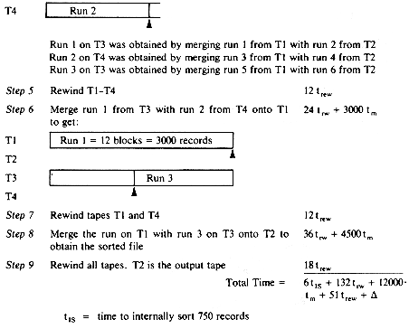
Example 8.3: A file containing 4,500 records, R1, ..., R4500 is to be sorted using a computer with an internal memory large enough to hold only 800 records. The available external storage consists of 4 tapes, T1, T2, T3 and T4. Each block on the input tape contains 250 records. The input tape is not to be destroyed during the sort. Initially, this tape is on one of the 4 available tape drives and so has to be dismounted and replaced by a work tape after all input records have been read. Let us look at the various steps involved in sorting this file. In order to simplify the discussion, we shall assume that the initial run generation is carried out using a conventional internal sort such as quicksort. In this case 3 blocks of input can be read in at a time, sorted and output as a run. We shall also assume that no parallelism in input, output and CPU processing is possible. In this case we shall use only one output buffer and two input buffers. This requires only 750 record spaces.
trw = time to read or write on block of 250 records onto tape starting at present position of read/write head
trew = time to rewind tape over a length correponding to 1 block
ntm = time to merge n records from input buffers to output buffer using a 2-way merge
The above computing time analysis assumes that no operations are carried out in parallel. The analysis could be carried out further as in the case of disks to show the dependence of the sort time on the number of passes made over the data.
Example 8.3 performed a 2-way merge of the runs. As in the case of disk sorting, the computing time here too depends essentially on the number of passes being made over the data. Use of a higher order merge results in a decrease in the number of passes being made without significantly changing the internal merge time. Hence, we would like to use as high an order merge as possible. In the case of disks the order of merge was limited essentially by the amount of internal memory available for use as input/output buffers. A k-way merge required the use of 2k + 2 buffers. While this is still true of tapes, another probably more severe restriction on the merge order k is the number of tapes available. In order to avoid excessive tape seek times, it is necessary that runs being merged together be on different tapes. Thus, a k-way merge requires at least k-tapes for use as input tapes during the merge.
In addition, another tape is needed for the output generated during this merge. Hence, at least k + 1 tapes must be available for a k-way tape merge (recall that in the case of a disk, one disk was enough for a k-way merge though two were needed to overlap input and output). Using k + 1 tapes to perform a k-way merge requires an additional pass over the output tape to redistribute the runs onto k-tapes for the next level of merges (see the merge tree of figure 8.8). This redistribution pass can be avoided through the use of 2k tapes. During the k-way merge, k of these tapes are used as input tapes and the remaining k as output tapes. At the next merge level, the role of input-output tapes is interchanged as in example 8.3, where in step 4, T1 and T2 are used as input tapes and T3 and T4 as output tapes while in step 6, T3 and T4 are the input tapes and T1 and T2 the output tapes (though there is no output for T2). These two approaches to a k-way merge are now examined. Algoritms M1 and M2 perform a k-way merge with the k + 1 tapes strategy while algorithm M3 performs a k-way merge using the 2k tapes strategy.
Analysis of Algorithm M1
To simplify the analysis we assume that the number of runs generated, m, is a power of k. Line 1 involves one pass over the entire file. One pass includes both reading and writing. In lines 5-11 the number of passes is logk m merge passes and logkm - 1 redistribution passes. So, the total number of passes being made over the file is 2logkm. If the time to rewind the entire input tape is trew, then the non-overlapping rewind time is roughly 2logkm trew.
A somewhat more clever way to tackle the problem is to rotate the output tape, i.e., tapes are used as output tapes in the cyclic order, k + 1,1,2, ...,k. When this is done, the redistribution from the output tape makes less than a full pass over the file. Algorithm M2 formally describes the process. For simplicity the analysis of M2 assumes that m is a power of k.
Analysis of Algorithm M2
The only difference between algorithms M2 and M1 is the redistributing
time. Once again the redistributing is done logkm - 1 times. m is the number of runs generated in line 1. But, now each redistributing pass reads and writes only (k - 1)/k of the file. Hence, the effective number of passes made over the data is (2 - 1/k)logkm + 1/k. For two-way merging on three tapes this means that algorithm M2 will make 3/2 logkm + 1/2 passes while M1 will make 2 logkm. If trew is the rewind time then the non-overlappable rewind time for M2 is at most (1 + 1/k) (logkm) trew + (1 - 1/k) trew as line 11 rewinds only 1/k of the file. Instead of distributing runs as in line 10 we could write the first m/k runs onto one tape, begin rewind, write the next m/k runs onto the second tape, begin rewind, etc. In this case we can begin filling input buffers for the next merge level (line 7) while some of the tapes are still rewinding. This is so because the first few tapes written on would have completed rewinding before the distribution phase is complete (for k > 2).
In case a k-way merge is made using 2k tapes, no redistribution is needed and so the number of passes being made over the file is only logkm + 1. This means that if we have 2k + 1 tapes available, then a 2k-way merge will make (2 - 1/(2k))log2km + 1/(2k) passes while a k-way merge utilizing only 2k tapes will make logkm + 1 passes. Table 8.13 compares the number of passes being made in the two methods for some values of k.
As is evident from the table, for k > 2 a k-way merge using only 2k tapes is better than a 2k-way merge using 2k + 1 tapes.
Algorithm M3 performs a k-way merge sort using 2k tapes.
Analysis of M3
To simplify the analysis assume that m is a power of k. In addition to the initial run creation pass, the algorithm makes logkm merge passes. Let trew be the time to rewind the entire input file. The time for line 2 is trew and if m is a power of k then the rewind of line 6 takes trew/k for each but the last iteration of the while loop. The last rewind takes time trew. The total rewind time is therefore bounded by (2 + (logkm - 1)/k)trew. Some of this may be overlapped using the strategy described in the analysis of algorithm M2 (exercise 4).
One should note that M1, M2 and M3 use the buffering algorithm of section 8.2.2 during the k-way merge. This merge itself, for large k, would be carried out using a selection tree as discussed earlier. In both cases the proper choice of buffer lengths and the merge order (restricted by the number of tape drives available) would result in an almost complete overlap of internal processing time with input/output time. At the end of each level of merge, processing will have to wait until the tapes rewind. Once again, this wait can be minimized if the run distribution strategy of exercise 4 is used.
Balanced k-way merging is characterized by a balanced or even distribution of the runs to be merged onto k input tapes. One consequence of this is that 2k tapes are needed to avoid wasteful passes over the data during which runs are just redistributed onto tapes in preparation for the next merge pass. It is possible to avoid altogether these wasteful redistribution passes, when using fewer than 2k tapes and a k-way merge, by distributing the "right number" of runs onto different tapes. We shall see one way to do this for a k-way merge utilizing k + 1 tapes. To begin, let us see how m = 21 runs may be merged using a 2-way merge with 3 tapes T1, T2 and T3. Lengths of runs obtained during the merge will be represented in terms of the length of initial runs created by the internal sort. Thus, the internal sort creates 21 runs of length 1 (the length of initial runs is the unit of measure). The runs on a tape will be denoted by sn where s is the run size and n the number of runs of this size. If there are six runs of length 2 on a tape we shall denote this by 26. The sort is carried out in seven phases. In the first phase the input file is sorted to obtain 21 runs. Thirteen of these are written onto T1 and eight onto T2. In phase 2, 8 runs from T2 are merged with 8 runs from T1 to get 8 runs of size 2 onto T3. In the next phase the 5 runs of length 1 from T1 are merged with 5 runs of length 2 from T3 to obtain 5 runs of length 3 on T2. Table 8.14 shows the 7 phases involved in the sort.
Counting the number of passes made during each phase we get 1 + 16/21 + 15/21 + 15/21 + 16/21 + 13/21 + 1 = 5-4/7 as the total number of passes needed to merge 21 runs. If algorithm M2 of section 8.3.1 had been used with k = 2, then 3/2
Table 8.15 shows the distribution of runs needed in each phase so that merging can be carried out without any redistribution passes. Thus, if we had 987 runs, then a distribution of 377 runs onto T1 and 610 onto T3 at phase 1 would result in a 15 phase merge. At the end of the fifteenth phase the sorted file would be on T1. No redistribution passes would have been made. The number of runs needed for a n phase merge is readily seen to be Fn + Fn-1 where Fi is the i-th Fibonacci number (recall that F7 = 13 and F6 = 8 and that F15 = 610 and F14 = 377). For this reason this method of distributing runs is also known as Fibonacci merge. It can be shown that for three tapes this distribution of runs and resultant merge pattern requires only 1.04 log2 m + 0.99 passes over the data. This compares very favorably with the log2 m passes needed by algorithm M3 on 4 tapes using a balanced 2-way merge. The method can clearly be generalized to k-way merging on k + 1 tapes using generalized Fibonacci numbers. Table 8.16 gives the run distribution for 3-way merging on four tapes. In this case it can be shown that the number of passes over the data is about 0.703 log2 m + 0.96.
Example 8.4: The initial internal sort of a file of records creates 57 runs. 4 tapes are available to carry out the merging of these runs. The table below shows the status of the tapes using 3-way polyphase merge.
The total number of passes over the data is 1 + 39/57 + 35/57 + 36/57 + 34/57 + 31/57 + 1 = 5-4/57 compared to [log257] = 6 passes for 2-way balanced merging on 4 tapes.
Remarks on Polyphase Merging
Our discussion of polyphase merging has ignored altogether the rewind time involved. Before one can begin the merge for the next phase it is necessary to rewind the output tape. During this rewind the computer is essentially idle. It is possible to modify the polyphase merge scheme discussed here so that essentially all rewind time is overlapped with internal processing and read/write on other tapes. This modification requires at least 5 tapes and can be found in Knuth Vol. 3. Further, polyphase merging requires that the initial number of runs be a perfect Fibonacci number (or generalized Fibonacci number). In case this is not so, one can substitute dummy runs to obtain the required number of runs.
Several other ingenious merge schemes have been devised for tape sorts. Knuth, Vol. 3, contains an exhaustive study of these schemes.
Both the balanced merge scheme of section 8.3.1 and the polyphase scheme of section 8.3.2 required at least 3 tapes to carry out the sort. These methods are readily seen to require only O(n log n) time where n is the number of records. We state without proof the following results for sorting on 1 and 2 tapes.
Theorem 8.2: Any one tape algorithm that sorts n records must take time
Theorem 8.3: n records can be sorted on 2 tapes in O(n log n) time if it is possible to perform an inplace rewrite of a record without destroying adjacent records. I.e. if record R2 in the sequence R1 R2 R3 can be rewritten by an equal size recod R'2 to obtain R1R'2R3.
See the readings for chapter 7.
The algorithm for theorem 8.3 may be found in:
"A linear time two tape merge" by R. Floyd and A. Smith, Information Processing Letters, vol. 2, no. 5, December 1973, pp. 123-126.
1. Write an algorithm to construct a tree of losers for records
2. Write an algorithm, using a tree of losers, to carry out a k-way merge of k runs
3. a) n records are to be sorted on a computer with a memory capacity of S records (S << n). Assume that the entire S record capacity may be used for input/output buffers. The input is on disk and consists of m runs. Assume that each time a disk access in made the seek time is ts and the latency time is tl. The transmission time is tt per record transmitted. What is the total input time for phase II of external sorting if a k way merge is used with internal memory partitioned into I/O buffers so as to permit overlap of input, output and CPU processings as in algorithm BUFFERING?
b) Let the CPU time needed to merge all the runs together be tCPU (we may assume it is independent of k and hence constant). Let ts = 80 ms, tl = 20 ms, n = 200,000, m = 64, tt = 10-3 sec/record, S = 2000. Obtain a rough plot of the total input time, tinput, versus k. Will there always be a value of k for which tCPU
4. a) Modify algorithm M3 using the run distribution strategy described in the analysis of algorithm M2.
b) et trw be the time to read/write a block and trew the time to rewind over one block length. If the initial run creation pass generates m runs for m a power of k, what is the time for a k-way merge using your algorithm. Compare this with the corresponding time for algorithm M2.
5. Obtain a table corresponding to Table 8.16 for the case of a 5-way polyphase merge on 6 tapes. Use this to obtain the correct initial distribution for 497 runs so that the sorted file will be on T1. How many passes are made over the data in achieving the sort? How many passes would have been made by a 5-way balanced merge sort on 6 tapes (algorithm M2)? How many passes would have been made by a 3-way balanced merge sort on 6 tapes (algorithm M3)?
6. In this exercise we shall investigate another run distribution strategy for sorting on tapes. Let us look at a 3-way merge on 4 tapes of 157 runs. These runs are initially distributed according to: 70 runs on T1, 56 on T2 and 31 on T3. The merging takes place according to the table below.
i.e., each phase consists of a 3-way merge followed by a two-way merge and in each phase almost all the initial runs are processed.
a) Show that the total number of passes made to sort 157 runs is 6-62/157.
b) Using an initial distribution from Table 8.16 show that Fibonacci merge on 4 tapes makes 6-59/193 passes when the number of runs is 193.
The distribution required for the process discussed above corresponds to the cascade numbers which are obtained as below for a k-way merge: Each phase (except the last) in a k-way cascade merge consists of a k-way merge followed by a k - 1 way merge followed by a k - 2 way merge . . . a 2-way merge. The last phase consists of only a k-way merge. The table below gives the cascade numbers corresponding to a k-way merge. Each row represents a starting configuration for a merge phase. If at the start of a phase we have the distribution n1, n2, ..., nk where ni > ni+ 1, 1
It can be shown that for a 4-way merge Cascade merge results in more passes over the data than a 4-way Fibonacci merge.
7. a) Generate the first 10 rows of the initial distribution table for a 5-way Cascade merge using 6 tapes (see exercise 6).
b) serve that 671 runs corresponds to a perfect 5-way Cascade distribution. How many passes are made in sorting the data using a 5-way Cascade merge?
c) How many passes are made by a 5-way Fibonacci merge starting with 497 runs and the distribution 120, 116, 108, 92, 61?
The number of passes is almost the same even though Cascade merge started with 35% more runs! In general, for
8. List the runs output by algorithm RUNS using the following input file and k = 4.
100,50, 18,60,2,70,30, 16,20, 19,99,55,20
9. For the example of Table 8.14 compute the total rewind time. Compare this with the rewind time needed by algorthm M2.
8.1 STORAGE DEVICES
8.1.1 Magnetic Tapes
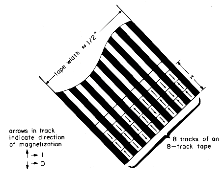
Figure 8.1 Segment of a Magnetic Tape
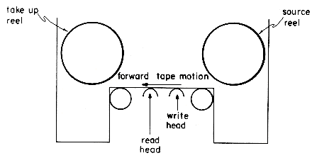
Figure 8.2 A Tape Drive
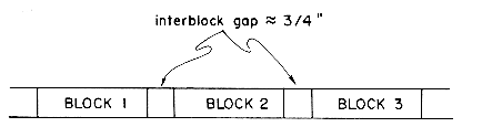
Figure 8.3 Blocked Data on a Tape
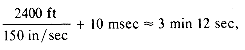 thus effecting an average transmission rate of almost 12 x 104 charac/sec. If, on the other hand, each block were one character long, then the tape would have at most 38,336 characters or blocks. This would be the worst case and the read time would be about 6 min 24 sec or an average of 100 charac/sec. Note that if the read of the next block is initiated soon enough after the read of the present block, then the delay time would be reduced to 5 milliseconds, corresponding to the time needed to get across the interblock gap of 3/4\" at a tape speed of 150 inches per second. In this case the time to read 38,336 one character blocks would be 3 min 12 sec, corresponding to an average of about 200 charac/sec.
8.1.2 Disk Storage
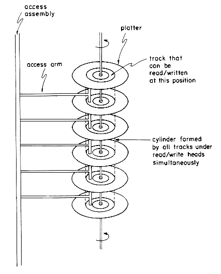
Figure 8.4 A Disk Drive with Disk Pack Mounted (Schematic).
8.2 SORTING WITH DISKS

Figure 8.5 Blocked Runs Obtained After Internal Sorting
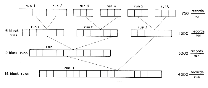
Figure 8.6 Merging the 6 runs
Operation Time
---------- ----
1) read 18 blocks of input, 18tIO, internally sort, 6tIS
write 18 blocks, 18tIO 36 tIO + 6 tIS
2) merge runs 1-6 in pairs 36 tIO + 4500 tm
3) merge 2 runs of 1500 records each, 12 blocks 24 tIO + 3000 tm
4) merge one run of 3000 records with one run of 1500
records 36 tIO + 4500 tm
--------------------------
Total Time 132 tIO + 12000 tm + 6 tIS
 12000 tm + 6 tIS.
8.2.1 k-Way Merging
 log2m
log2m + 1 levels for a total of log2m passes over the data file. The number of passes over the data can be reduced by using a higher order merge, i.e., k-way merge for k
  2. In this case we would simultaneously merge k runs together. Figure 8.7 illustrates a 4-way merge on 16 runs. The number of passes over the data is now 2, versus 4 passes in the case of a 2-way merge. In general, a k-way merge on m runs requires at most logkm passes over the data. Thus, the input/output time may be reduced by using a higher order merge. The use of a higher order merge, however, has some other effects on the sort. To begin with, k-runs of size S1, S2, S3, ...,Sk can no longer be merged internally in
  time. In a k-way merge, as in a 2-way merge, the next record to be output is the one with the smallest key. The smallest has now to be found from k possibilities and it could be the leading record in any of the k-runs. The most direct way to merge k-runs would be to make k - 1 comparisons to determine the next record to output. The computing time for this would be
  . Since logkm passes are being made, the total number of key comparisons being made is n(k - 1) logkm = n(k - 1) log2m/log2k where n is the number of records in the file. Hence, (k - 1)/log2k is the factor by which the number of key comparisons increases. As k increases, the reduction in input/output time will be overweighed by the resulting increase in CPU time needed to perform the k-way merge. For large k (say, k 6) we can achieve a significant reduction in the number of comparisons needed to find the next smallest element by using the idea of a selection tree. A selection tree is a binary tree where each node represents the smaller of its two children. Thus, the root node represents the smallest node in the tree. Figure 8.9 illustrates a selection tree for an 8-way merge of 8-runs.
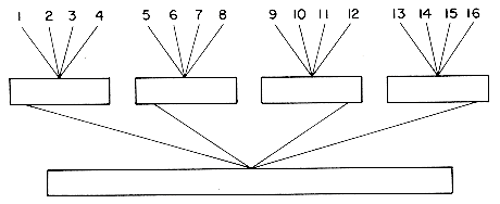
Figure 8.7 A 4-way Merge on 16 Runs
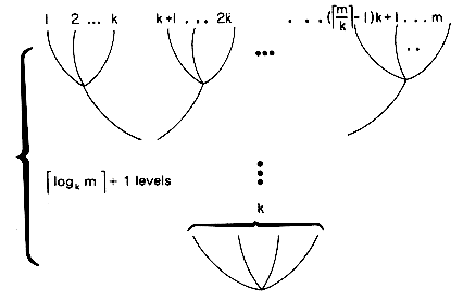
Figure 8.8 A k-Way Merge
log2k + 1. So, the time to restructure the tree is O(log2k). The tree has to be restructured each time a record is merged into the output file. Hence, the time required to merge all n records is O(n log2k). The time required to set up the selection tree the first time is O(k). Hence, the total time needed per level of the merge tree of figure 8.8 is O(n log2k). Since the number of levels in this tree is O(logkm), the asymptotic internal processing time becomes O(n log2k logkm) = O(n log2 m). The internal processing time is independent of k.
Figure 8.9 Selection tree for 8-way merge showing the first three keys in each of the 8 runs.
Figure 8.10 Selection tree of Figure 8.9 after one record has been output and tree restructured. Nodes that were changed are marked by
 .
.
Figure 8.11 Tree of Losers Corresponding to Figure 8.9
8.2.2 Buffer Handling for Parallel Operation
 i 4, and two output buffers, OU(1) and OU(2). Each buffer is capable of holding two records. The first few records of run 1 have key value 1, 3, 5, 7, 8, 9. The first few records of run 2 have key value 2, 4, 6, 15, 20, 25. Buffers IN(1) and IN(3) are assigned to run 1. The remaining two input buffers are assigned to run 2. We start the merging by reading in one buffer load from each of the two runs. At this time the buffers have the configuration of figure 8.12(a). Now runs 1 and 2 are merged using records from IN (1) and IN(2). In parallel with this the next buffer load from run 1 is input. If we assume that buffer lengths have been chosen such that the times to input, output and generate an output buffer are all the same then when OU(1) is full we have the situation of figure 8.12(b). Next, we simultaneously output OU(1), input into IN(4) from run 2 and merge into OU(2). When OU(2) is full we are in the situation of figure 8.12(c). Continuing in this way we reach the configuration of figure 8.12(e). We now begin to output OU(2), input from run 1 into IN(3) and merge into OU(1). During the merge, all records from run 1 get exhausted before OU(1) gets full. The generation of merged output must now be delayed until the inputting of another buffer load from run 1 is completed!
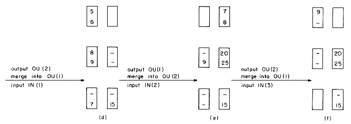
Figure 8.12 Example showing that two fixed buffers per run are not enough for continued parallel operation
 , using a k-way merge. 2k input buffers and 2 output buffers are used. Each buffer is a contiguous block of memory. Input buffers are queued in k queues, one queue for each run. It is assumed that each input/output buffer is long enough to hold one block of records. Empty buffers are stacked with AV pointing to the top buffer in this stack. The stack is a linked list. The following variables are made use of:
 IN (i) ... input buffers, 1
i 2k OUT (i) ... output buffers, 0
i 1FRONT (i) ... pointer to first buffer in queue for run i, 1
i k END (i) ... end of queue for i-th run, 1
i k LINK (i) ... link field for i-th input buffer
in a queue or for buffer in stack 1
i 2k LAST (i) ... value of key of last record read
from run i, 1
i k OU ... buffer currently used for output.
 . If block lengths and hence buffer lengths are chosen such that the time to merge one output buffer load equals the time to read a block then almost all input, output and computation will be carried out in parallel. It is also assumed that in the case of equal keys the k-way merge algorithm first outputs the record from the run with smallest index.
 procedure BUFFERING
1 for i <-- 1 to k do //input a block from each run//
2 input first block of run i into IN(i)
3 end
4 while input not complete do end //wait//
5 for i <-- 1 to k do //initialize queues and free buffers//
6 FRONT(i) <-- END(i) <-- i
7 LAST(i) <-- last key in buffer IN(i)
8 LINK(k + i) <-- k + i + 1 //stack free buffer//
9 end
10 LINK(2k) <-- 0; AV <-- k + 1; OU <-- 0
//first queue exhausted is the one whose last key read is smallest//
11 find j such that LAST(j) = min {LAST(i)} l
ik12 l <-- AV; AV <-- LINK(AV) //get next free buffer//
13 if LAST(j)
 + then [begin to read next block for run j into
 buffer IN(l)]
14 repeat //KWAYMERGE merges records from the k buffers
FRONT(i) into output buffer OU until it is full.
If an input buffer becomes empty before OU is filled, the
next buffer in the queue for this run is used and the empty
buffer is stacked or last key = +
//15 call KWAYMERGE
16 while input/output not complete do //wait loop//
17 end
if LAST(j)
+ then18 [LINK(END(j)) <-- l; END(j) <-- l; LAST(j) <-- last key read
//queue new block//
19 find j such that LAST(j) = min {LAST(i)} l
ik20 l <-- AV; AV <-- LINK(AV)] //get next free buffer//
21 last-key-merged <-- last key in OUT(OU)
22 if LAST(j)
+ then [begin to write OUT(OU) and read next block of run j into IN(l)]
23 else [begin to write OUT(OU)]
24 OU <-- 1 - OU
25 until last-key-merged = +
26 while output incomplete do //wait loop//
27 end
28 end BUFFERING
i k, rather than making k - 1 comparisons each time a buffer load is to be read in. The change in computing time will not be significant, since this queue selection represents only a very small fraction of the total time taken by the algorithm. we begin reading one by one the first blocks from each of the next set of k runs to be merged. In this case, over the entire sorting of a file, the only time that is not overlapped with the internal merging time is the time for the first k blocks of input and that for the last block of output.. . We have six input buffers IN(i), 1 i 6, and 2 output buffers OUT(0) and OUT(1). The diagram on page 404 shows the status of the input buffer queues, the run from which the next block is being read and the output buffer being ouput at the beginning of each iteration of the repeat-until of the buffering algorithm (lines 14-25). since otherwise KWAYMERGE would terminate the search rather then get another buffer for Ri. This means that there are more blocks of records for run Ri on the input file and LAST(i) +. Consequently, up to this time whenever a block was output another was simultaneously read in (see line 22). Input/output therefore proceeded at the same rate and the number of available blocks of data is always k. An additional block is being read in but it does not get queued until line 18. Since the queue for Ri has become empty first, the selection rule for the next run to read from ensures that there is at most one block of records for each of the remaining k - 1 runs. Furthermore, the output buffer cannot be full at this time as this condition is tested for before the input buffer empty condition. Thus there are fewer than k blocks of data in memory. This contradicts our earlier assertion that there must be exactly k such blocks of data.
 8.2.3 Run Generation
i < k. This will require a loser tree with k nodes numbered 0 to k - 1. Each node, i, in this tree will have one field L (i). L(i), 1 i < k represents the loser of the tournament played at node i. Node 0 represents the overall winner of the tournament. This node will not be explicitly present in the algorithm. Each of the k record positions R (i), has a run number field RN (i), 0 i < k associated with it. This field will enable us to determine whether or not R (i) can be output as part of the run currently being generated. Whenever the tournament winner is output, a new record (if there is one) is input and the tournament replayed as discussed in section 8.2.1. Algorithm RUNS is simply an implementation of the loser tree strategy discussed earlier. The variables used in this algorithm have the following significance: R(i), 0
i < k ... the k records in the tournament treeKEY(i), 0
i < k ... key value of record R(i) L(i), 0 < i < k ... loser of the tournament played at node i
RN(i), 0 <= i < k ... the run number to which R(i) belongs
RC ... run number of current run
Q ... overall tournament winner
RQ ... run number for R(Q)
RMAX ... number of runs that will be generated
LAST__KEY ... key value of last record output
 i sets up a loser tree with R(0) the winner. With this initialization the loop of lines 5-26 correctly sets up the loser tree for run 1. The test of line 10 suppresses the output of these k fictitious records making up run 0. The variable LAST__KEY is made use of in line 13 to determine whether or not the new record input, R(Q), can be output as part of the current run. If KEY(Q) < LAST__KEY then R(Q) cannot be output as part of the current run RC as a record with larger key value has already been output in this run. When the tree is being readjusted (lines 18-24), a record with lower run number wins over one with a higher run number. When run numbers are equal, the record with lower key value wins. This ensures that records come out of the tree in nondecreasing order of their run numbers. Within the same run, records come out of the tree in nondecreasing order of their key values . RMAX is used to terminate the algorithm. In line 11, when we run out of input, a record with run number RMAX + 1 is introduced. When this record is ready for output, the algorithm terminates in line 8. One may readily verify that when the input file is already sorted, only one run is generated. On the average, the run size is almost 2k. The time required to generate all the runs for an n run file is O(n log k) as it takes O(log k) time to adjust the loser tree each time a record is output. The algorithm may be speeded slightly by explicitly initializing the loser tree using the first k records of the input file rather than k fictitious records as in lines 1-4. In this case the conditional of line 10 may be removed as there will no longer be a need to suppress output of certain records.
8.3 SORTING WITH TAPES
procedure RUNS
//generate runs using a tree of losers//
1 for i
1 to k - 1 do //set up fictitious run 0 to initializetree//
2 RN(i)
0; L(i) i; KEY(i) 03 end
4 Q
RQ RC RMAX RN(0) 0; LAST__KEY 5 loop //output runs//
6 if RQ
RC then [//end of run//7 if RC
0 then output end of run marker8 if RQ > RMAX then stop
9 else RC
RQ]//output record R(Q) if not fictitious//
10 if RQ
0 then [output R(Q); LAST__KEY KEY (Q)]//input new record into tree//
11 if no more input then [RQ
RMAX + 1; RN (Q) RQ]12 else [input a new record into R (Q)
13 if KEY (Q) < LAST__KEY
14 then [//new record belongs to next
run//
15 RQ
RQ + 116 RN (Q)
RQRMAX
RQ]17 else [RN (Q)
RC]]//adjust losers//
18 T
 (k + Q)/2
 //T is parent of Q//
19 while T
0 do20 if RN (L(T)) < RQ or (RN(L(T)) = RQ and KEY(L(T)) <
KEY(Q))
21 then [TEMP
Q; Q L(T); L(T) TEMP//T is the winner//
22 RQ
RN(Q)]23 T
T/2 //move up tree//24 end
25 forever
26 end RUNS
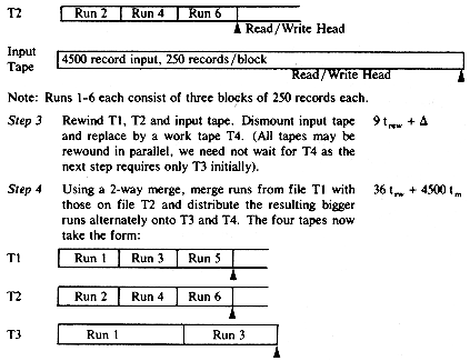
 = delay cause by having to wait for T4 to be mounted in case we are ready to use T4 in step 4 before the completion of this tape mount.
8.3.1 Balanced Merge Sorts
procedure M1
//Sort a file of records from a given input tape using a k-way
merge given tapes T1, ...,Tk+1 are available for the sort.//
1 Create runs from the input file distributing them evenly over
tapes T1, ...,Tk
2 Rewind T1, ...,Tk and also the input tape
3 if there is only 1 run then return //sorted file on T1//
4 replace input tape by Tk+1
5 loop //repeatedly merge onto Tk+1 and redistribute back
onto T1, ...,Tk//
6 merge runs from T1, ...,Tk onto Tk+1
7 rewind T1, ....,Tk+1
8 if number of runs on Tk+1 = 1 then return //output on
Tk+1//
9 evenly distribute from Tk+1 onto T1, ...,Tk
10 rewind T1, ...,Tk+1
11 forever
12 end M1
procedure M2
//same function as M1//
1 Create runs from the input tape, distributing them evenly over
tapes T1, ...,Tk.
2 rewind T1, ...,Tk and also the input tape
3 if there is only 1 run then return //sorted file is on T1//
4 replace input tape by Tk+1
5 i
k + 1 //i is index of output tape//6 loop
7 merge runs from the k tapes Tj, 1
j k + 1 and j i ontoTi
8 rewind tapes T1, ...,Tk+1
9 if number of runs on Ti = 1 then return //output on Ti//
10 evenly distribute (k - 1)/k of the runs on Ti onto tapes Ti, 1
j
k +1 and j i and j i mod(k + 1) + 111 rewind tapes Tj, 1
j k + 1 and j i12 i
i mod(k + 1) + 113 forever
14 end M2
k 2k-way k-way
1 3/2 log2 m + 1/2 --
2 7/8 log2 m + 1/6 log2 m + 1
3 1.124 log3 m + 1/6 log3 m + 1
4 1.25 log4 m + 1/8 log4 m + 1
Table 8.13 Number of passes using a 2k-way merge versus a k-way merge on 2k + 1 tapes
procedure M3
//Sort a file of records from a given input tape using a k-way
merge on 2k tapes T1, ...,T2k//
1 Create runs from the input file distributing them evenly over tapes
T1, ...,Tk
2 rewind T1, ...,Tk; rewind the input tape; replace the input tape by
tape T2k; i
03 while total number of runs on Tik+1, ...,Tik+k > 1 do
4 j
1 - i5 perform a k-way merge from Tik+1, ...,Tik+k evenly distributing
output runs onto Tjk+1, ...,Tjk+k.
6 rewind T1, ...,T2k
7 i
j //switch input an output tapes//8 end
//sorted file is on Tik+1//
9 end M3
8.3.2 Polyphase Merge
Fraction of
Total Records
Phase T1 T2 T3 Read
1 113 18 -- 1 initial distribution
2 15 -- 28 16/21 merge to T3
3 -- 35 23 15/21 merge to T2
4 53 32 -- 15/21 merge to T1
5 51 -- 82 16/21 merge to T3
6 -- 131 81 13/21 merge to T2
7 211 -- -- 1 merge to T1
Table 8.14 Polyphase Merge on 3 Tapes
log221 + 1/2 = 8 passes would have been made. Algorithm M3 using 4 tapes would have made log221 = 5 passes. What makes this process work? Examination of Table 8.14 shows that the trick is to distribute the runs initially in such a way that in all phases but the last only 1 tape becomes empty. In this case we can proceed to the next phase without redistribution of runs as we have 2 non-empty input tapes and one empty tape for output. To determine what the correct initial distribution is we work backwards from the last phase. Assume there are n phases. Then in phase n we wish to have exactly one run on T1 and no runs on T2 and T3. Hence, the sort will be complete at phase n. In order to achieve this, this run must be obtained by merging a run from T2 with a run from T3, and these must be the only runs on T2 and T3. Thus, in phase n - 1 we should have one run on each of T2 and T3. The run on T2 is obtained by merging a run from T1 with one from T3. Hence, in phase n - 2 we should have one run on T1 and 2 on T3.Phase T1 T2 T3
n 1 0 0
n - 1 0 1 1
n - 2 1 0 2
n - 3 3 2 0
n - 4 0 5 3
n - 5 5 0 8
n - 6 13 8 0
n - 7 0 21 13
n - 8 21 0 34
n - 9 55 34 0
n - 10 0 89 55
n - 11 89 0 144
n - 12 233 144 0
n - 13 0 377 233
n - 14 377 0 610
Table 8.15 Run Distribution for 3-Tape Polyphase Merge
Phase T1 T2 T3 T4
n 1 0 0 0
n - 1 0 1 1 1
n - 2 1 0 2 2
n - 3 3 2 0 4
n - 4 7 6 4 0
n - 5 0 13 11 7
n - 6 13 0 24 20
n - 7 37 24 0 44
n - 8 81 68 44 0
n - 9 0 149 125 81
n - 10 149 0 274 230
n - 11 423 274 0 504
n - 12 927 778 504 0
n - 13 0 1705 1431 927
n - 14 1705 0 3136 2632
Table 8.16 Polyphase Merge Pattern for 3-Way 4-Tape Merging
Fraction of
Total Records
Phase T1 T2 T3 T4 Read
1 113 -- 124 120 1 initial distribution
2 -- 313 111 17 39/57 merge onto T2
3 57 36 14 -- 35/57 merge onto T1
4 53 32 -- 94 36/57 merge onto T4
5 51 -- 172 92 34/57 merge onto T3
6 -- 311 171 91 31/57 merge onto T2
7 571 -- -- -- 1 merge onto T1
8.3.3 Sorting with Fewer Than 3 Tapes
O(n2).REFERENCES
EXERCISES
 with key values
  . Let the tree nodes be
  with
with  a pointer to the loser of a tournament and T0 a pointer to the overall winner. Show that this construction can be carried out in time O(k).
 . Show that if there are n records in the k runs together, then the computing time is O(n log2k). tinput?
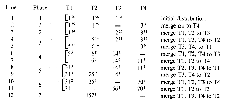 i < k, then at the start of the previous phase we need
  runs on the k input tapes respectively.
Initial Distribution for a k-way Cascade Merge

 6 tapes Cascade merge makes fewer passes over the data than does Fibonacci merge.