Is a symbol table necessarily a set of names or can the same name appear more than once? If we are translating a language with block structure (such as ALGOL or PL/I) then the variable X may be declared at several levels. Each new declaration of .X implies that a new variable (with the same name) must be used. Thus we may also need a mechanism to determine which of several occurrences of the same name has been the most recently introduced.
These considerations lead us to a specificaton of the structure symbol table. A set of axioms are given on the next page.
Imagine the following set of declarations for a language with block structure:
begin
integer i,j;
.
.
.
begin
real x,i;
.
.
The representation of the symbol table for these declarations would look like S =
INSERT(INSERT(INSERT(INSERT(CREATE,i,integer),
j,integer),x,real),i,real)
Notice the identifer i which is declared twice with different attributes. Now suppose we apply FIND (S,i). By the axioms EQUAL(i,i) is tested and has the value true. Thus the value real is returned as a result. If the function DELETE(S,i) is applied then the result is the symbol table
INSERT(INSERT(INSERT(CREATE,i,integer),j,integer),x,real)
If we wanted to change the specification of DELETE so that it removes all occurrences of i then one axiom needs to be redefined, namely
The remaining sections of this chapter are organized around different ways to implement symbol tables. Different strategies are preferable given different assumptions. The first case considered is where the identifiers are known in advance and no deletions or insertions are allowed. Symbol tables with this property are called static. One solution is to sort the names and store them sequentially. Using either the binary search or Fibonacci search method of section 7.1 allows us to find any name in O(log2n) operations. If each name is to be searched for with equal probability then this solution, using an essentially balanced binary search tree, is optimal. When different identifiers are searched for with differing probabilities and these probabilities are known in advance this solution may not be the best. An elegant solution to this problem is given in section 9.1.
In section 9.2 we consider the use of binary trees when the identifiers are not known in advance. Sequential allocation is no longer desirable because of the need to insert new elements. The solution which is examined is AVL or height balanced trees. Finally in section 9.3 we examine the most practical of the techniques for dynamic search and insertion, hashing.
Definition: A binary search tree T is a binary tree; either it is empty or each node in the tree contains an identifier and:
(i) all identifiers in the left subtree of T are less (numerically or alphabetically) than the identifier in the root node T;
(ii) all identifiers in the right subtree of T are greater than the identifier in the root node T;
(iii) the left and right subtrees of T are also binary search trees.
For a given set of identifiers several binary search trees are possible. Figure 9.1 shows two possible binary search trees for a subset of the reserved words of SPARKS.
To determine whether an identifier X is present in a binary search tree, X is compared with the root. If X is less than the identifier in the root, then the search continues in the left subtree; if X equals the identifier in the root, the search terminates successfully; otherwise the search continues in the right subtree. This is formalized in algorithm SEARCH.
In our study of binary search in chapter 7, we saw that every sorted file corresponded to a binary search tree. For instance, a binary search on the file (do, if, stop) corresponds to using algorithm SEARCH on the binary search tree of figure 9.2. While this tree is a full binary tree, it need not be optimal over all binary search trees for this file when the identifiers are searched for with different probabilities. In order to determine an optimal binary search tree for a given static file, we must first decide on a cost measure for search trees. In searching for an identifier at level k using algorithm SEARCH, k iterations of the while loop of lines 2-8 are made. Since this loop determines the cost of the search, it is reasonable to use the level number of a node as its cost.
Consider the two search trees of figure 9.1 as possibly representing the symbol table of the SPARKS compiler. As names are encountered a match is searched for in the tree. The second binary tree requires at most three comparisons to decide whether there is a match. The first binary tree may require four comparisons, since any identifier which alphabetically comes after if but precedes repeat will test four nodes. Thus, as far as worst case search time is concerned, this makes the second binary tree more desirable than the first. To search for an identifier in the first tree takes one comparison for the if, two for each of for and while, three for repeat and four for loop. Assuming each is searched for with equal probability, the average number of comparisons for a successful search is 2.4. For the second binary search tree this amount is 2.2. Thus, the second tree has a better average behavior, too.
In evaluating binary search trees, it is useful to add a special "square" node at every place there is a null link. Doing this to the trees of figure 9.1 yields the trees of figure 9.3. Remember that every binary tree with n nodes has n + 1 null links and hence it will have n + 1 square nodes. We shall call these nodes external nodes because they are not part of the original tree. The remaining nodes will be called internal nodes. Each time a binary search tree is examined for an identifier which is not in the tree, the search terminates at an external node. Since all such searches represent unsuccessful searches, external nodes will also be referred to as failure nodes. A binary tree with external nodes added is an extended binary tree. Figure 9.3 shows the extended binary trees corresponding to the search trees of figure 9.1. We define the external path length of a binary tree to be the sum over all external nodes of the lengths of the paths from the root to those nodes. Analogously, the internal path length is defined to be the sum over all internal nodes of the lengths of the paths from the root to those nodes. For the tree of figure 9.3(a) we obtain its internal path length, I, to be:
I = 0 + 1 + 1 + 2 + 3 = 7
Its external path length, E, is:
E = 2 + 2 + 4 + 4 + 3 + 2 = 17.
Exercise 1 shows that the internal and external path lengths of a binary tree with n internal nodes are related by the formula E = I + 2n. Hence, binary trees with the maximum E also have maximum I. Over all binary trees with n internal nodes what are the maximum and minimum possible values for I? The worst case, clearly, is when the tree is skewed (i.e., when the tree has a depth of n). In this case,
To obtain trees with minimal I, we must have as many internal nodes as close to the root as possible. We can have at most 2 nodes at distance 1, 4 at distance 2, and in general the smallest value for I is
0 + 2
This can be more compactly written as
One tree with minimal internal path length is the complete binary tree defined in section 5.2.
Before attempting to use these ideas of internal and external path length is to obtain optimal binary search trees, let us look at a related but simpler problem. We are given a set of n + 1 positive weights q1, ...,qn + 1. Exactly one of these weights is to be associated with each of the n + 1 external nodes in a binary tree with n internal nodes. The weighted external path length of such a binary tree is defined to be
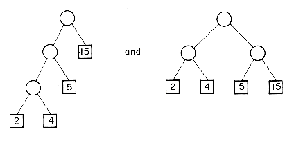
For example, suppose n = 3 and we are given the four weights: q1 = 15, q2 = 2, q3 = 4 and q4 = 5. Two possible trees would be:
Their respective weighted external path lengths are:
2
and
2
Binary trees with minimal weighted external path length find application in several areas. One application is to determine an optimal merge pattern for n + 1 runs using a 2-way merge. If we have four runs R1-R4 with qi being the number of records in run Ri, 1
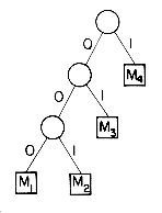
Another application of binary trees with minimal external path length is to obtain an optimal set of codes for messages M1, ...,Mn + 1. Each code is a binary string which will be used for transmission of the corresponding message. At the receiving end the code will be decoded using a decode tree. A decode tree is a binary tree in which external nodes represent messages. The binary bits in the code word for a message determine the branching needed at each level of the decode tree to reach the correct external node. For example, if we interpret a zero as a left branch and a one as a right branch, then the decode tree corresponds to codes 000, 001, 01 and 1 for messages M1, M2, M3 and M4 respectively. These codes are called Huffman codes. The cost of decoding a code word is proportional to the number of bits in the code. This number is equal to the distance of the corresponding external node from the root node. If qi is the relative frequency with which message Mi will be transmitted, then the expected decode time is
A very nice solution to the problem of finding a binary tree with minimum weighted external path length has been given by D. Huffman. We simply state his algorithm and leave the correctness proof as an exercise. The algorithm HUFFMAN makes use of a list L of extended binary trees. Each node in a tree has three fields: WEIGHT, LCHILD and RCHILD. Initially, all trees in L have only one node. For each tree this node is an external node, and its weight is one of the provided qi's. During the course of the algorithm, for any tree in L with root node T and depth greater than 1, WEIGHT(T) is the sum of weights of all external nodes in T. Algorithm HUFFMAN uses the subalgorithms LEAST and INSERT. LEAST determines a tree in L with minimum WEIGHT and removes it from L. INSERT adds a new tree to the list L.
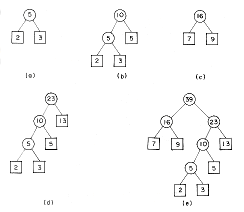
We illustrate the way this algorithm works by an example. Suppose we have the weights q1 = 2, q2 = 3, q3 = 5, q4 = 7, q5 = 9 and q6 = 13. Then the sequence of trees we would get is: (the number in a circular node represents the sum of the weights of external nodes in that subtree).
The weighted external path length of this tree is
2
In comparison, the best complete binary tree has weighted path length 95.
The main loop is executed n - 1 times. If L is maintained as a heap (section 7.6) then each call to LEAST and INSERT requires only O(log n) time. Hence, the asymptotic computing time for the algorithm is O(n log n).
Let us now return to our original problem of representing a symbol table as a binary search tree. If the binary search tree contains the identifiers a1,a2, ...,an with a1 < a2 < ... < an and the probability of searching for each ai is pi, then the total cost of any binary search tree is
An optimal binary search tree for the identifier set a1, ...,an is one which minimizes eq. (9.1) over all possible binary search trees for this identifier set. Note that since all searches must terminate either successfully or unsuccessfully we have
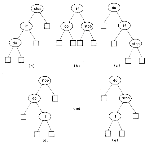
Example 9.1: The possible binary search trees for the identifier set (a1,a2,a3) = (do, if, stop) are:
With equal probabilities pi = qj = 1/7 for all i and j we have:
As expected, tree b is optimal. With p1 = .5, p2 = .1, p3 = .05, q0 = .15, q1 = .1, q2 = .05 and q3 = .05 we have
Tree c is optimal with this assignment of p's and q's.
From among all the possible binary search trees how does one determine the optimal tree? One possibility would be to proceed as in example 9.1 and explicitly generate all possible binary search trees. The cost of each such tree could be computed and an optimal tree determined. The cost of each of the binary search trees can be determined in time O(n) for an n node tree. If N(n) is the total number of distinct binary search trees with n identifiers, then the complexity of the algorithm becomes O(n N(n)). From section 5.9 we know that N(n) grows too rapidly with increasing n to make this brute force algorithm of any practical significance. Instead we can find a fairly efficient algorithm by making some observations regarding the properties of optimal binary search trees.
Let a1 < a2 < ... < an be the n identifiers to be represented in a binary search tree. Let us denote by Tij an optimal binary search tree for ai+1, ...,aj, i < j. We shall adopt the convention that Tii is an empty tree for 0
If Tij is an optimal binary search tree for ai+1, ...,aj and rij = k, i < k
From eq. (9.2) it is clear that if cij is to be minimal, then cost (L) = ci,k-1 and cost (R) = ck,j as otherwise we could replace either L or R by a subtree of lower cost thus getting a binary search tree for ai+1, ...,aj with lower cost than cij. This would violate the assumption that Tij was optimal. Hence, eq. (9.2) becomes:
Since Tij is optimal it follows from eq. (9.3) that rij = k is such that
or
Equation (9.4) gives us a means of obtaining Ton and con starting from the knowledge that Tii =
Example 9.2: Let n = 4 and (a1, a2, a3, a4) = (do, if, read, while). Let (p1, p2, p3, p4) = (3,3,1,1) and (q0, q1, q2, q3, q4) = (2,3,1,1,1). The p's and q's have been multiplied by 16 for convenience. Initially, we have wi,i = qi, cii = 0 and rii = 0, 0
Knowing wi,i + 1 and ci,i + 1, 0
The above example illustrates how equation (9.4) may be used to determine the c's and r's and also how to reconstruct Ton knowing the r's. Let us examine the complexity of this procedure to evaluate the c's and r's. The evaluation procedure described in the above example requires us to compute cij for (j - i) = 1,2, ...,n in that order. When j - i = m there are n - m + 1 cij's to compute. The computation of each of these cij's requires us to find the minimum of m quantities (see equation (9.4)). Hence, each such cij can be computed in time O(m). The total time for all cij's with j - i = m is therefore O(nm - m2). The total time to evaluate all the cij's and rij's is therefore
Actually we can do better than this using a result due to D. E. Knuth which states that the optimal l in equation (9.4) may be found by limiting the search to the range ri,j-1
Dynamic tables may also be maintained as binary search trees. An identifier X may be inserted into a binary search tree T by using the search algorithm of the previous section to determine the failure node corresponding to X. This gives the position in T where the insertion is to be made. Figure 9.7 shows the binary search tree obtained by entering the months JANUARY to DECEMBER in that order into an initially empty binary search tree. Algorithm BST is a more formal rendition of the insertion process just described.
The maximum number of comparisons needed to search for any identifier in the tree of figure 9.7 is six for NOVEMBER. The average number of comparisons is (1 for JANUARY + 2 each for FEBRUARY and MARCH + 3 each for APRIL, JUNE and MAY + ... + 6 for NOVEMBER) / 12 = 42/ 12 = 3.5. If the months are entered in the order JULY, FEBRUARY, MAY, AUGUST, DECEMBER, MARCH, OCTOBER, APRIL, JANUARY, JUNE, SEPTEMBER and NOVEMBER then the tree of figure 9.8 is obtained. This tree is well balanced and does not have any paths to a node with a null link that are much longer than others. This is not true of the tree of figure 9.7 which has six nodes on the path from the root to NOVEMBER and only two nodes, JANUARY and FEBRUARY, on another path to a null link. Moreover, during the construction of the tree of figure 9.8 all intermediate trees obtained are also well balanced. The maximum number of identifier comparisons needed to find any identifier is now 4 and the average is 37/12
From our earlier study of binary trees, we know that both the average and maximum search time will be minimized if the binary search tree is maintained as a complete binary tree at all times. However, since we are dealing with a dynamic situation, identifiers are being searched for while the table is being built and so it is difficult to achieve this ideal without making the time required to add new entries very high. This is so because in some cases it would be necessary to restructure the whole tree to accommodate the new entry and at the same time have a complete binary search tree. It is, however, possible to keep the trees balanced so as to ensure both an average and worst case retrieval time of O(log n) for a tree with n nodes. We shall study one method of growing balanced binary trees. These balanced trees will have satisfactory search and insertion time properties.
Adelson-Velskii and Landis in 1962 introduced a binary tree structure that is balanced with respect to the heights of subtrees. As a result of the balanced nature of this type of tree, dynamic retrievals can be performed in O(log n) time if the tree has n nodes in it. At the same time a new identifier can be entered or deleted from such a tree in time O(log n). The resulting tree remains height balanced. The tree structure introduced by them is given the name AVL-tree. As with binary trees it is natural to define AVL trees recursively.
Definition: An empty tree is height balanced. If T is a nonempty binary tree with TL and TR as its left and right subtrees, then T is height balanced iff (i) TL and TR are height balanced and (ii) |hL - hR|
The definition of a height balanced binary tree requires that every subtree also be height balanced. The binary tree of figure 9.7 is not height balanced since the height of the left subtree of the tree with root 'APRIL' is 0 while that of the right subtree is 2. The tree of figure 9.8 is height balanced while that of figure 9.9 is not. To illustrate the processes involved in maintaining a height balanced binary search tree, let us try to construct such a tree for the months of the year. This time let us assume that the insertions are made in the order MARCH, MAY, NOVEMBER, AUGUST, APRIL, JANUARY, DECEMBER, JULY, FEBRUARY, JUNE, OCTOBER and SEPTEMBER. Figure 9.10 shows the tree as it grows and the restructuring involved in keeping the tree balanced. The numbers within each node represent the difference in heights between the left and right subtrees of that node. This number is referred to as the balance factor of the node.
Definition: The balance factor, BF(T), of a node T in a binary tree is defined to be hL - hR where hL and hR are the heights of the left and right subtrees of T. For any node T in an AVL tree BF(T) = - 1, 0 or 1.
Inserting MARCH and MAY results in the binary search trees (i) and (ii) of figure 9.10. When NOVEMBER is inserted into the tree the height of the right subtree of MARCH becomes 2, while that of the left subtree is 0. The tree has become unbalanced. In order to rebalance the tree, a rotation is performed. MARCH is made the left child of MAY and MAY becomes the root. The introduction of AUGUST leaves the tree balanced. However, the next insertion, APRIL, causes the tree to become unbalanced again. To rebalance the tree, another rotation is performed. This time, it is a clockwise rotation. MARCH is made the right child of AUGUST and AUGUST becomes the root of the subtree (figure 9.10(v)). Note that both the previous rotationswere carried out with respect to the closest parent of the new node having a balance factor of
In the preceding example we saw that the addition of a node to a balanced binary search tree could unbalance it. The rebalancing was carried out using essentially four different kinds of rotations LL, RR, LR and RL (figure 9.10 (v), (iii), (vi) and (ix) respectively). LL and RR are symmetric as are LR and RL. These rotations are characterized by the nearest ancestor, A, of the inserted node, Y, whose balance factor becomes
LL: new node Y is inserted in the left subtree of the left subtree of A
LR: Y is inserted in the right subtree of the left subtree of A
RR: Y is inserted in the right subtree of the right subtree of A
RL: Y is inserted in the left subtree of the right subtree of A
Figures 9.11 and 9.12 show these rotations in terms of abstract binary trees. The root node in each of the trees of the figures represents the nearest ancestor whose balance factor has become
In order to be able to carry out the rebalancing of figures 9.11 and 9.12 it is necessary to locate the node A around which the rotation is to be performed. As remarked earlier, this is the nearest ancestor of the newly inserted node whose balance factor becomes
In order to really understand the insertion algorithm, the reader should try it out on the example of figure 9.10. Once you are convinced that it does keep the tree balanced, then the next question is how much time does it take to make an insertion? An analysis of the algorithm reveals that if h is the height of the tree before insertion, then the time to insert a new identifier is O(h). This is the same as for unbalanced binary search trees, though the overhead is significantly greater now. In the case of binary search trees, however, if there were n nodes in the tree, then h could in the worst case be n (figure 9.9) and the worst case insertion time was O(n). In the case of AVL trees, however, h can be at most O(log n) and so the worst case insertion time is O(log n). To see this, let Nh be the minimum number of nodes in a height balanced tree of height h. In the worst case, the height of one of the subtrees will be h - 1 and of the other h - 2. Both these subtrees are also height balanced. Hence, Nh = Nh-1 + Nh-2 + 1 and N0 = 0, N1 = 1 and N2 = 2. Note the similarity between this recursive definition for Nh and that for the Fibonacci numbers Fn = Fn-1 + Fn-2, F0 = 0 and F1 = 1. In fact, we can show (exercise 16) that Nh = Fh+2 - 1 for h
Exercises 9-13 show that it is possible to find and delete a node with identifier X and to find and delete the kth node from a height balanced tree in O(log n) time. Results of an empirical study of deletion in height balanced trees may be found in the paper by Karlton, et.al. (see the references). Their study indicates that a random insertion requires no rebalancing, a rebalancing rotation of type LL or RR and a rebalancing rotation of type LR and RL with probabilities .5349, .2327 and .2324 respectively. Table 9.12 compares the worst case times of certain operations on sorted sequential lists, sorted linked lists and AVL-trees. Other suitable balanced tree schemes are studied in Chapter 10.
In tree tables, the search for an identifier key is carried out via a sequence of comparisons. Hashing differs from this in that the address or location of an identifier, X, is obtained by computing some arithmetic function, f, of X. f(X) gives the address of X in the table. This address will be referred to as the hash or home address of X. The memory available to maintain the symbol table is assumed to be sequential. This memory is referred to as the hash table, HT. The hash table is partitioned into b buckets, HT(0), ...,HT(b - 1). Each bucket is capable of holding s records. Thus, a bucket is said to consist of s slots, each slot being large enough to hold 1 record. Usually s = 1 and each bucket can hold exactly 1 record. A hashing function, f(X), is used to perform an identifier transformation on X. f(X) maps the set of possible identifiers onto the integers 0 through b - 1. If the identifiers were drawn from the set of all legal Fortran variable names then there would be T =
As an example, let us consider the hash table HT with b = 26 buckets, each bucket having exactly two slots, i.e., s = 2. Assume that there are n = 10 distinct identifiers in the program and that each identifier begins with a letter. The loading factor,
In summary, hashing schemes perform an identifier transformation through the use of a hash function f. It is desirable to choose a function f which is easily computed and also minimizes the number of collisions. Since the size of the identifier space, T, is usually several orders of magnitude larger than the number of buckets b, and s is small, overflows necessarily occur. Hence a mechanism to handle overflows is also needed.
A hashing function, f, transforms an identifier X into a bucket address in the hash table. As mentioned earlier the desired properties of such a function are that it be easily computable and that it minimize the number of collisions. A function such as the one discussed earlier is not a very good choice for a hash function for symbol tables even though it is fairly easy to compute. The reason for this is that it depends only on the first character in the identifier. Since many programs use several identifiers with the same first letter, we expect several collisions to occur. In general, then, we would like the function to depend upon all the characters in the identifiers. In addition, we would like the hash function to be such that it does not result in a biased use of the hash table for random inputs. I.e., if X is an identifier chosen at random from the identifier space, then we want the probability that f(X) = i to be 1/b for all buckets i. Then a random X has an equal chance of hashing into any of the b buckets. A hash function satisfying this property will be termed a uniform hash function.
Several kinds of uniform hash functions are in use. We shall describe four of these.
(i) Mid-Square
One hash function that has found much use in symbol table applications is the 'middle of square' function. This function,
(ii) Division
Another simple choice for a hash function is obtained by using the modulo (mod) operator. The identifier X is divided by some number M and the remainder is used as the hash address for X.
fD(X) = X mod M
This gives bucket addresses in the range 0 - (M - 1) and so the hash table is at least of size b = M. The choice of M is critical. If M is a power of 2, then fD(X) depends only on the least significant bits of X. For instance, if each character is represented by six bits and identifiers are stored right justified in a 60-bit word with leading bits filled with zeros (figure 9.15) then with M = 2i, i
Let us try some other values for M and see what kind of identifiers get mapped to the same bucket. The goal being that we wish to avoid a choice of M that will lead to many collisions. This kind of an analysis is possible as we have some idea as to the relationships between different variable names programmers tend to use. For instance, the knowledge that a program tends to have variables with the same suffix led us to reject M = 2i. For similar reasons even values of M prove undesirable. Let X = x1x2 and Y = x2x1 be two identifiers each consisting of the characters x1 and x2. If the internal binary representation of x1 has value C(x1) and that for x2 has value C(x2) then if each character is represented by 6 bits, the numeric value of X is 26C(x1) + C(x2) while that for Y is 26C(x2) + C(x1). If p is a prime number dividing M then (fD(X) - fD(Y)) mod p = (26C(x1)mod p + C(x2)mod p - 26C(X2)mod p - C(x1)mod p) mod p. If p = 3, then
I.e., permutations of the same set of characters are hashed at a distance a factor of 3 apart. Programs in which many variables are permutations of each other would again result in a biased use of the table and hence result in many collisions. This happens because 64 mod 3 = 1. The same behavior can be expected when 7 divides M as 64 mod 7 = 1. These difficulties can be avoided by choosing M a prime number. Then, the only factors of M are M and 1. Knuth has shown that when M divides rk
(iii) Folding
In this method the identifier X is partitioned into several parts, all but the last being of the same length. These parts are then added together to obtain the hash address for X. There are two ways of carrying out this addition. In the first, all but the last part are shifted so that the least significant bit of each part lines up with the corresponding bit of the last part (figure 9.16(a)). The different parts are now added together to get f(X). This method is known as shift folding. The other method of adding the parts is folding at the boundaries. In this method, the identifier is folded at the part boundaries and digits falling into the same position are added together (figure 9.16(b)) to obtain f(X).
(iv) Digit Analysis
This method is particularly useful in the case of a static file where all the identifiers in the table are known in advance. Each identifier X is interpreted as a number using some radix r. The same radix is used for all the identifiers in the table. Using this radix, the digits of each identifier are examined. Digits having the most skewed distributions are deleted. Enough digits are deleted so that the number of digits left is small enough to give an address in the range of the hash table. The criterion used to find the digits to be used as addresses, based on the measure of uniformity in the distribution of values in each digit, is to keep those digits having no abnormally high peaks or valleys and those having small standard deviation. The same digits are used for all identifiers.
Experimental results presented in section 9.3.2 suggest the use of the division method with a divisor M that has no prime factors less than 20 for general purpose applications.
In order to be able to detect collisions and overflows, it is necessary to initialize the hash table, HT, to represent the situation when all slots are empty. Assuming that no record has identifier zero, then all slots may be initialized to zero.* When a new identifier gets hashed into a full bucket, it is necessary to find another bucket for this identifier.The simplest solution would probably be to find the closest unfilled bucket. Let us illustrate this on a 26-bucket table with one slot per bucket. Assume the identifiers to be GA, D, A, G, L, A2, A1, A3, A4, Z, ZA, E. For simplicity we choose the hash function f(X) = first character of X. Initially, all the entries in the table are zero. f(GA) = 7, this bucket is empty, so GA and any other information making up the record are entered into HT(7). D and A get entered into the buckets HT(4) and HT(1) respectively. The next identifier G has f(G) = 7. This slot is already used by GA. The next vacant slot is HT(8) and so G is entered there. L enters HT(12). A2 collides with A at HT(1), the bucket overflows and A2 is entered at the next vacant slot HT(2). A1, A3 and A4 are entered at HT(3), HT(5) and HT(6) respectively. Z is entered at HT(26), ZA at HT(9), (the hash table is used circularly), and E collides with A3 at HT(5) and is eventually entered at HT(10). Figure 9.17 shows the resulting table. This method of resolving overflows is known as linear probing or linear open addressing.
*A clever way to avoid initializing the hash table has been discovered by T. Gonzalez (see exercise 22).
In order to search the table for an identifier, X, it is necessary to first compute f(X) and then examine keys at positions HT(f(X)), HT(f(X) + 1), ...,HT(f(X) + j) such that HT(f(X) + j) either equals X (X is in the table) or 0 (X is not in the table) or we eventually return to HT(f(X)) (the table is full).
Our earlier example shows that when linear probing is used to resolve overflows, identifiers tend to cluster together, and moreover, adjacent clusters tend to coalesce, thus increasing the search time. To locate the identifier, ZA, in the table of figure 9.17, it is necessary to examine HT(26), HT(1), ...,HT(9), a total of ten comparisons. This is far worse than the worst case behavior for tree tables. If each of the identifiers in the table of figure 9.12 was retrieved exactly once, then the number of buckets examined would be 1 for A, 2 for A2, 3 for A1, 1 for D, 5 for A3, 6 for A4, 1 for GA, 2 for G, 10 for ZA, 6 for E, 1 for L and 1 for Z for a total of 39 buckets examined. The average number examined is 3.25 buckets per identifier. An analysis of the method shows that the expected average number of identifier comparisons, P, to look up an identifier is approximately (2 -
One of the problems with linear open addressing is that it tends to create clusters of identifiers. Moreover, these clusters tend to merge as more identifiers are entered, leading to bigger clusters. Some improvement in the growth of clusters and hence in the average number of probes needed for searching can be obtained by quadratic probing. Linear probing was characterized by searching the buckets (f(X) + i) mod b; 0
One of the reasons linear probing and its variations perform poorly is that searching for an identifier involves comparison of identifiers with different hash values. In the hash table of figure 9.17, for instance, searching for the identifier ZA involved comparisons with the buckets HT(1) to HT(8), even though none of the identifiers in these buckets had a collision with HT(26) and so could not possibly be ZA. Many of the comparisons being made could be saved if we maintained lists of identifiers, one list per bucket, each list containing all the synonyms for that bucket. If this were done, a search would then involve computing the hash address f(X) and examining only those identifiers in the list for f(X). Since the sizes of these lists is not known in advance, the best way to maintain them is as linked chains. Additional space for a link is required in each slot. Each chain will have a head node. The head node, however, will usually be much smaller than the other nodes since it has to retain only a link. Since the lists are to be accessed at random, the head nodes should be sequential. We assume they are numbered 1 to M if the hash function f has range 1 to M.
Using chaining to resolve collisions and the hash function used to obtain figure 9.17, the hash chains of figure 9.19 are obtained. When a new identifier, X, is being inserted into a chain, the insertion can be made at either end. This is so because the address of the last node in the chain is known as a result of the search that determined X was not in the list for f(X). In the example of figure 9.19 new identifiers were inserted at the front of the chains. The number of probes needed to search for any of the identifiers is now 1 for each of A4, D, E, G, L, and ZA; 2 for each of A3, GA and Z; 3 for A1: 4 for A2 and 5 for A for a total of 24. The average is now 2 which is considerably less than for linear probing. Additional storage, however, is needed for links.
The expected number of identifier comparison can be shown to be
The results of this section tend to imply that the performance of a hash table depends only on the method used to handle overflows and is independent of the hash function so long as a uniform hash function is being used. While this is true when the identifiers are selected at random from the identifier space, it is not true in practice. In practice, there is a tendency to make a biased use of identifiers. Many identifiers in use have a common suffix or prefix or are simple permutations of other identifiers. Hence, in practice we would expect different hash functions to result in different hash table performance. The table of figure 9.20 presents the results of an empirical study conducted by Lum, Yuen and Dodd. The values in each column give the average number of bucket accesses made in searching eight different tables with 33,575; 24,050; 4909; 3072; 2241; 930; 762 and 500 identifiers each. As expected, chaining outperforms linear open addressing as a method for overflow handling. In looking over the figures for the various hash functions, we see that division is generally superior to the other types of hash functions. For a general application, it is therefore recommended that the division method be used. The divisor should be a prime number, though it is sufficient to choose a divisor that has no prime factors less than 20. The table also gives the theoretical expected number of bucket accesses based on random keys.
The experimental evaluation of hashing techniques indicates a very good performance over conventional techniques such as balanced trees. The worst case performance for hashing can, however, be very bad. In the worst case an insertion or a search in a hash table with n identifiers may take O(n) time. In this section we present a probabilistic analysis for the expected performance of the chaining method and state without proof the results of similar analyses for the other overflow handling methods. First, we formalize what we mean by expected performance.
Let HT(0: b - 1) be a hash table with b buckets, each bucket having one slot. Let f be a uniform hash function with range [0, b - 1]. If n identifiers X1,X2,...,Xn are entered into the hash table then there are bn distinct hash sequences f(X1), f(X2), ...,f(Xn). Assume that each of these is equally likely to occur. Let Sn denote the expected number of identifier comparisons needed to locate a randomly chosen Xi, 1
Theorem 9.1 Let
(i) for linear open addressing
(ii) for rehashing, random probing and quadratic probing
(iii) for chaining
Un
Sn
Proof Exact derivations of Un and Sn are fairly involved and can be found in Knuth's book: The Art of Computer Programming: Sorting and Searching. Here, we present a derivation of the approximate formulas for chaining. First, we must make clear our count for Un and Sn. In case the identifier X being searched for has
When the n identifiers distribute uniformly over the b possible chains, the expected number in each chain is n/b=
When the i'th identifier, Xi, is being entered into the table, the expected number of identifiers on any chain is (i - 1)/b. Hence, the expected number of comparisons needed to search for Xi after all n identifiers have been entered is 1 + (i - 1)/b (this assumes that new entries will be made at the end of the chain). We therefore get:
The O(n2) optimum binary search tree algorithm is from:
"Optimum Binary Search Trees" by D. Knuth, Acta Informatica, vol. 1, Fasc 1, 1971, pp. 14-25.
For a discussion of heuristics that obtain in O(nlogn) time nearly optimal binary search trees see:
"Nearly Optimal Binary Search Trees," by K. Melhorn, Acta Informatica, vol. 5, pp. 287-295, 1975.
"Binary Search Trees and File Organization," by J. Nievergelt, ACM Computing Surveys, vol. 6, no. 3, Sept. 1974, pp. 195-207.
For more on Huffman codes see: An Optimum Encoding with Minimum Longest Code and Total Number of Digits, by E. Schwartz, Information and Control, vol. 7, 1964, pp. 37-44.
Additional algorithms to manipulate AVL trees may be found in:
"Linear lists and priority queues as balanced binary trees" by C. Crane, STAN-CS-72-259, Computer Science Department, Stanford University, February 1972.
The art of computer programming: sorting and searching by D.Knuth, Addiso-Wesley, Reading, Massachusetts. 1973 (section 6.2.3).
Results of an empirical study on height balanced trees appear in:
"Performance of Height-Balanced Trees," by P. L. Karlton, S. H. Fuller, R. E. Scroggs and E. B. Koehler, CACM, vol. 19, no. 1, Jan. 1976, pp. 23-28.
Several interesting and enlightening works on hash tables exist. Some of these are:
"Scatter storage techniques" by R. Morris, CACM, vol. 11, no. 1, January 1968, pp. 38-44.
"Key to Address Transform Techniques: A Fundamental Performance Study on Large Existing Formatted Files" by V. Lum, P. Yuen and M. Dodd, CACM, vol. 14, no. 4, April 1971, pp. 228-239.
"The quadratic quotient method: a hash code eliminating secondary clustering" by J. Bell, CACM, vol. 13, no. 2, February 1970, pp. 107-109.
"Full table quadratic searching for scatter storage" by A. Day, CACM, vol. 13, no. 8, August 1970, pp. 481-482.
"Identifier search mechanisms: a survey and generalized model" by D. Severence, ACM Computing Surveys, vol. 6, no. 3, September 1974, pp. 175-194.
"A practitioners guide to addressing algorithms: a collection of reference tables and rules-of-thumb" by D. Severence and R. Duhne, Technical Report No. 240, Department of Operations Research, Cornell University, November 1974.
"Hash table methods" by W. Mauer and T. Lewis, ACM Computing Surveys, vol. 7, no. 1, March 1975, pp. 5-20.
"The quadratic hash method when the table size is not prime" by V. Batagelj, CACM, vol. 18, no. 4, April 1975, pp. 216-217.
The art of computer programming: sorting and searching by D. Knuth, Addison-Wesley, Reading, Massachusetts, 1973.
"Reducing the retrieval time of scatter storage techniques" by R. Brent, CACM, vol. 16, no. 2, February 1973, pp. 105-109.
"General performance analysis of key-to-address transformation methods using an abstract file concept" by V. Lum, CACM, vol. 16, no. 10, October 1973, pp. 603-612.
"The use of quadratic residue research," by C. E. Radke, CACM, vol. 13, no. 2, Feb. 1970, pp. 103-105.
A method to avoid hash table initialization may be found in:
"Algorithms for sets and related problems," by T. Gonzalez, University of Oklahoma, Nov. 1975.
1. (a) Prove by induction that if T is a binary tree with n internal nodes, I its internal path length and E its external path length, then E = I + 2n, n
(b) Using the result of (a) show that the average number of comparisons s in a successful search is related to the average number of comparisons, u, in an unsuccessful search by the formula
s = (1 + 1/n)u - 1, n
2. (a) Show that algorithm HUFFMAN correctly generates a binary tree of minimal weighted external path length.
(b) When n runs are to be merged together using an m-way merge, Huffman's method generalizes to the following rule: "First add (1 - n) mod (m - 1) runs of length zero to the set of runs. Then repeatedly merge together the m shortest remaining runs until only one run is left." Show that this rule yields an optimal merge pattern for m-way merging.
3. Using algorithm OBST compute wij, rij and cij, 0
4. (a) Show that the computing time of algorithm OBST is O(n2).
(b) Write an algorithm to construct the optimal binary search tree Ton given the roots rij, 0
5. Since, often, only the approximate values of the p's and q's are known, it is perhaps just as meaningful to find a binary search tree that is nearly optimal i.e. its cost, eq. (9.1), is almost minimal for the given p's and q's. This exercise explores an O(nlogn) algorithm that results in nearly optimal binary search trees. The search tree heuristic we shall study is:
Choose the root Ak such that | w0,k - 1 - wk,n| is as small as possible. Repeat this procedure to find the left and right subtrees of Ak.
(a) Using this heuristic obtain the resulting binary search tree for the data of exercise 3. What is its cost?
(b) Write a SPARKS algorithm implementing the above heuristic. Your algorithm should have a time complexity of at most O(n log n).
An analysis of the performance of this heuristic may be found in the paper by Melhorn.
6. (a) Convince yourself that Figures 9.11 and 9.12 take care of all the possible situations that may arise when a height balanced binary tree becomes unbalanced as a result of an insertion. Alternately come up with an example that is not covered by any of the cases in Figures 9.11 and 9.12.
(b) Complete Figure 9.12 by drawing the tree configurations for the rotations RL (a), (b) and (c).
7. Complete algorithm AVL--INSERT by filling in the steps needed to rebalance the tree in case the imbalance was of type RL.
8. Obtain the height balanced trees corresponding to those of Figure 9.10 using algorithm AVL--INSERT, starting with an empty tree, on the following sequence of insertions:
DECEMBER, JANUARY, APRIL, MARCH, JULY, AUGUST, OCTOBER, FEBRUARY, NOVEMBER, MAY, JUNE.
Label the rotations according to type.
9. Assume that each node in an AVL tree T has the field LSIZE. For any node, A, LSIZE(A) is the number of nodes in its left subtree +1. Write an algorithm AVL--FINDK(T,k) to locate the kth smallest identifier in the subtree T. Show that this can be done in O(log n) time if there are n nodes in T.
10. Rewrite algorithm AVL--INSERT with the added assumption that each node has a LSIZE field as in exercise 9. Show that the insertion time remains O(log n).
11. Write an algorithm to list the nodes of an AVL-tree T in ascending order of IDENT fields. Show that this can be done in O(n) time if T has n nodes.
12. Write an algorithm to delete the node with identifier X from an AVL-tree T. The resulting tree should be restructured if necessary. Show that the time required for this is O(log n) when there are n nodes in T.
13. Do exercise 12 for the case when each node has a LSIZE field and the kth smallest identifier is to be deleted.
14. Write an algorithm to merge the nodes of the two AVL-trees T1 and T2 together. What is the computing time of your algorithm?
15. Write an algorithm to split an AVL tree, T, into two AVL trees T1 and T2 such that all identifiers in T1 are
16. Prove by induction that the minimum number of nodes in an AVL tree of height h is Nh = Fh+2 - 1, h
17. Write an algorithm to delete identifier X from a hash table which uses hash function f and linear open addressing to resolve collisions. Show that simply setting the slot previously occupied by X to 0 does not solve the problem. How must algorithm LINSRCH be modified so that a correct search is made in the situation when deletions are permitted? Where can a new identifier be inserted?
18. (i) Show that if quadratic searching is carried out in the sequence (f(x) + q2), f(x) + (q - 1)2),...,(f(x) + 1),f(x),(f(x) - 1), ...,(f(x) - q2) with q = (b - 1)12 then the address difference mod b between successive buckets being examined is
b - 2, b - 4, b - 6, ...,5, 3, 1, 1, 3, 5, ...,b - 6, b - 4, b - 2
(ii) Write an algorithm to search a hash table HT (0,b - 1) of size b for the identifier X. Use f as the hash function and the quadratic probe scheme discussed in the text to resolve. In case X is not in the table, it is to be entered. Use the results of part (i) to reduce the computations.
19. [Morris 1968] In random probing, the search for an identifier, X, in a hash table with b buckets is carried out by examining buckets f(x), f(x) + S(i), 1
Initialize R to 1 each time the search routine is called.
On successive calls for a random number do the following:
R
R
S(i)
(ii) Write an algorithm, incorporating the above random number generator, to search and insert into a hash table using random probing and the middle of square hash function, fm.
It can be shown that for this method, the expected value for the average number of comparisons needed to search for X is - (1/
20. Write an algorithm to list all the identifiers in a hash table in lexicographic order. Assume the hash function f is f(X) = first character of X and linear probing is used. How much time does your algorithm take?
21. Let the binary representation of identifier X be x1x2. Let | x | denote the number of bits in x and let the first bit of x1 be 1. Let | x1 | =
f(X) = middle k bits of (x1 XOR x2)
where XOR is exclusive or. Is this a uniform hash function if identifiers are drawn at random from the space of allowable FORTRAN identifiers? What can you say about the behavior of this hash function in a real symbol table usage?
22. [T. Gonzalez] Design a symbol table representation which allows one to search, insert and delete an identifier X in O(1) time. Assume that 1
23. [T. Gonzalez] Let S = {x1,x2, ...,xn} and T = {y1,y2, ...,yr} be two sets. Assume 1
24. [T. Gonzalez] Using the idea of exercise 22 write an O(n + m) time algorithm to carry out the function of algorithm VERIFY2 of section 7.1. How much space does your algorithm need?
25. Complete table 9.12 by adding a column for hashing.
26. For a fixed k, k
Definition An empty binary tree is a HB(k) tree. If T is a non-empty binary tree with TL and TR as its left and right subtrees, then T is HB(k) iff (i) TL and TR are HB(k) and (ii) | hL - hR |
For the case of HB(2) trees obtain the rebalancing transformations.
27. Write an insertion algorithm for HB(2) trees.
28. Using the notation of section 9.3.3 show that when linear open addressing is used:
Using this equation and the approximate equality:
29. [Guttag] The following set of operations define a symbol table which handles a language with block structure. Give a set of axioms for these operations:
INIT--creates an empty table;
ENTERB--indicates a new block has been entered;
ADD--places an identifier and its attributes in the table;
LEAVEB--deletes all identifiers which are defined in the innermost block;
RETRIEVE--returns the attributes of the most recently defined identifier;
ISINB--returns true if the identifier is defined in the innermost block else false.
DELETE(INSERT(S,a,r),b) :: =
if EQUAL(a,b) then DELETE(S,b)
else INSERT(DELETE(S,b),a,r)
structure SYMBOL__TABLE
declare CREATE( )
 symtb
symtbINSERT(symtb,name, value)
 symtb
symtbDELETE(symtb,name)
 symtb
symtbFlND(symtb,name)
 value
valueHAS(symtb,name)
 Boolean
ISMTST(symtb)
 Boolean;
for all S
 symtb, a,b
  name, r
  value let
ISMTST(CREATE) :: = true
ISMTST(INSERT(S,a,r)) :: = false
HAS(CREATE,a) :: = false
HAS(INSERT(S,a,r),b) :: =
if EQUAL(a,b) then true else HAS(S,b)
DELETE(CREATE,a) :: = CREATE
DELETE(INSERT(S,a,r),b) :: =
if EQUAL(a,b) then S
else INSERT(DELETE(S,b),a,r)
FIND(CREATE,a) :: = error
FIND(INSERT(S,a,r),b) :: = if EQUAL(a,b) then r
else FIND(S,b)
end
end SYMBOL__TABLE
9.1 STATIC TREE TABLES
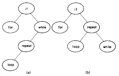
Figure 9.1 Two possible binary search trees
procedure SEARCH(T,X,i)
//search the binary search tree T for X. Each node has fields
LCHILD, IDENT, RCHILD. Return i = 0 if X is not in T.
Otherwise, return i such that IDENT(i) = X.//
1 i
 T
T2 while i
 0 do
0 do3 case
4 :X < IDENT(i): i
 LCHILD(i) //search left subtree//
5 :X = IDENT(i): return
6 :X > IDENT(i): i
 RCHILD(i) //search right subtree//
7 end
8 end
9 end SEARCH
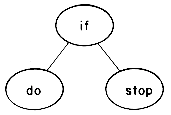
Figure 9.2 Binary search tree corresponding to a binary search on the file (do,if,stop).
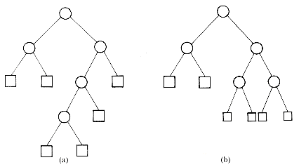
Figure 9.3 Extended binary trees corresponding to search trees of figure 9.1.

 1 + 4
1 + 4  2 + 8
2 + 8  3 + ....
 1
1 i
i n + 1 qi ki where ki is the distance from the root node to the external node with weight qi. The problem is to determine a binary tree with minimal weighted external path length. Note that here no information is contained within internal nodes.
 3 + 4
3 + 4  3 + 5
3 + 5  2 + 15
  1 = 43
 2 + 4
2 + 4  2 + 5
2 + 5  2 + 15
  2 = 52.
 i
i  4, then the skewed binary tree above defines the following merge pattern: merge R2 and R3; merge the result of this with R4 and finally merge with R1. Since two runs with n and m records each can be merged in time O(n + m) (cf., section 7.5), the merge time following the pattern of the above skewed tree is proportional to (q2 + q3) + {(q2 + q3) + q4} + {q1 + q2 + q3 + q4}. This is just the weighted external path length of the tree. In general, if the external node for run Ri is at a distance ki from the root of the merge tree, then the cost of the merge will be proportional to
  qiki which is the weighted external path length.
 1
1 i
i n + 1 qidi where di is the distance of the external node for message Mi from the root node. The expected decode time is minimized by choosing code words resulting in a decode tree with minimal weighted external path length!
procedure HUFFMAN(L,n)
//L is a list of n single node binary trees as described above//
for i
 1 to n - 1 do //loop n - 1 times//
call GETNODE(T) //create a new binary tree//
LCHILD(T)
 LEAST(L) //by combining the trees//
RCH1LD(T)
 LEAST(L) //with the two smallest weights//
WEIGHT(T)
 WEIGHT(LCHILD(T))
+ WEIGHT(RCHILD(T))
call INSERT(L,T)
end
end HUFFMAN
 4 + 3
4 + 3  4 + 5
4 + 5  3 + 13
  2 + 7
2 + 7  2 + 9
2 + 9  2 = 93
Analysis of Algorithm HUFFMAN
 1
1 i
i n pi. level (ai) when only successful searches are made. Since unsuccessful searches, i.e., searches for identifiers not in the table, will also be made, we should include the cost of these searches in our cost measure, too. Unsuccessful searches terminate with i = 0 in algorithm SEARCH. Every node with a null subtree defines a point at which such a termination can take place. Let us replace every null subtree by a failure node. The identifiers not in the binary search tree may be partitioned into n + 1 classes Ei, 0
  i
i  n. Eo contains all identifiers X such that X< a1. Ei contains all identifiers X such that ai < X < ai+1, 1
  i < n and En contains all identifiers X, X > an. It is easy to see that for all identifiers in a particular class Ei, the search terminates at the same failure node and it terminates at different failure nodes for identifiers in different classes. The failure nodes may be numbered 0 to n with i being the failure node for class Ei, 0
  i
i  n. If qi is the probability that the identifier being searched for is in Ei, then the cost of the failure nodes is
  0
0 i
i n qi; (level (failure node i) - 1). The total cost of a binary search tree is therefore:
(9.1)
 1
1 i
i n Pi +
  0
0 i
i n qi = 1.
cost (tree a) = 15/7; cost (tree b) = 13/7
cost (tree c) = 15/7; cost (tree d) = 15/7
cost (tree e) = 15/7.
cost (tree a) = 2.65; cost (tree b) = 1.9
cost (tree c) = 1.5; cost (tree d) = 2.05
cost (tree e) = 1.6
 i
i  n and that Tij is not defined for i > j. We shall denote by cij the cost of the search tree Tij. By definition cii will be 0. rij will denote the root of Tij and wij = qi +
  jk=i+1 (qk + pk) will denote the weight of Tij. By definition we will have rii = 0 and wii = qi, 0
  i
i  n. An optimal binary search tree for a1, ...,an is therefore Ton, its cost is con, its weight won and its root ron.
 j, then Tij has two subtrees L and R. L is the left subtree and contains the identifiers ai+1, ...,ak-1 and R is the right subtree and contains the identifiers ak+1, ...,aj (figure 9.4). The cost cij of Tij is
ci,j = pk + cost (L) + cost (R) + wi,k-1+ wk,j
weight (L) = weight (Ti,k-1) = wi,k-1
weight (R) = weight (Tk,j) = wk,j
(9.2)
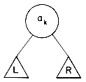
Figure 9.4 An optimal binary search tree Tij
ci,j = pk + wi,k-1 + wk,j + ci,k-1 + ck,j
= wi,j + ci,k-1 + ck,j
(9.3)
wij + ci,k-1 + ck,j = min {wij + ci,l-1 + cl,j}i<l
 j
jci,k-1 + ck,j = min {ci,1-1 + cl,j}i<l
 j
j(9.4)
 and cii = 0.
 i
i  4. Using eqs. (9.3) and (9.4)we get:
w01 = p1 + w00 + w11 = p1 + q1 + w00 = 8
c01 = w01 + min {c00 + c11} = 8r01 = 1
w12 = p2 + w11 + w22 = p2 + q2 + w11 = 7
c12 = w12 + min {c11 + c22} = 7r12 = 2
w23 = p3 + w22 + w33 = p3 + q3 + w22 = 3
c23 = w23 + min {c22 + c33} = 3r23 = 3
w34 = p4 + w33 + w44 = p4 + q4 + w33 = 3
c34 = w34 + min {c33 + c44} = 3r34= 4
 i
i  4 we can again use equations (9.3) and (9.4)to compute wi,i + 2, ci,i + 2, ri,i + 2, 0
  i
i  3. This process may be repeated until w04, c04 and r04 are obtained. The table of figure 9.5 shows the results of this computation. From the table we see that c 04 = 32 is the minimal cost of a binary search tree for a1 to a4. The root of tree T04 is a2. Hence, the left subtree is T01 and the right subtree T24. T01 has root a1 and subtrees T00 and T11. T24 has root a3; its left subtree is therefore T22 and right subtree T34. Thus, with the data in the table it is possible to reconstruct T04. Figure 9.6 shows T04.
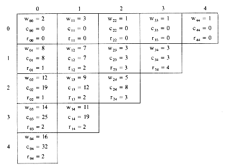
Figure 9.5 Computation of c04, w04 and r04. The computation is carried out row wise from row 0 to row 4.

Figure 9.6 Optimal search tree for example 9.2
 1
1 m
m n (nm - m2) = O(n3).
 l
l  ri+1,j. In this case the computing time becomes O(n2) (exercise 4). Algorithm OBST uses this result to obtain in O(n2) time the values of wij, rij and cij, 0
  i
i  j
j  n. The actual tree Ton may be constructed from the values of rij in O(n) time. The algorithm for this is left as an exercise.
procedure OBST(pi,qi,n)
//Given n distinct identifiers a1 < a2 < ... < an and probabilities pi,
1
 i
i  n and qi, 0
  i
i  n this algorithm computes the cost cij
of optimal binary search trees Tij for identifiers ai+1, ...,aj.
It also computes rij, the root of Tij. wij is the weight of Tij//
for i
 0 to n - 1 do
(wii,rii,cii)
 (qi,0,0) //initialize//
(wi,i+1,ri,i+1,ci,i+1)
 (qi + qi+1 + pi+1, i+1, qi+ qi+1 + pi+1)
//optimal trees with one node//
end
(wnn,rnn,cnn)
 (qn,0,0)
for m
 2 to n do //find optimal trees with m nodes//
for i
 0 to n - m do
j
 i + m
i + mwij
 wi,j-1 + pj + qj
k
 a value of l in the range ri,j-1
  l
l  ri+1,j
that minimizes {ci,l-1 +cl,j} //solve (9.4) usingKnuth's result//
cij
 wij + ci,k-1 + ck,j //eq. (9.3)//
rij
 k
kend
end
end OBST
9.2 DYNAMIC TREE TABLES
 3.1. If instead the months are entered in lexicographic order, the tree degenerates to a chain as in figure 9.9. The maximum search time is now 12 identifier comparisons and the average is 6.5. Thus, in the worst case, binary search trees correspond to sequential searching in an ordered file. When the identifiers are entered in a random order, the tree tends to be balanced as in figure 9.8. If all permutations are equiprobable then it can be shown the average search and insertion time is O(log n) for an n node binary search tree.
procedure BST (X,T,j)
//search the binary search tree T for the node j such that IDENT(j)
= X. If X is not already in the table then it is entered at the
appropriate point. Each node has LCHILD, IDENT and RCHILD
fields//
p
 0; j
0; j  T //p will trail j through the tree//
while j
 0 do
0 docase
:X < IDENT(j): p
 j; j
j; j  LCHILD(j) //search left
sub-tree//
:X = IDENT(j): return
:X > IDENT(j): p
 j; j
j; j  RCHILD(j) //search right
sub-tree//
end
end
//X is not in the tree and can be entered as a child of p//
call GETNODE(j); IDENT(j)
 X; LCHILD(j)
  0;
0;RCHILD(j)
 0
0case
:T = 0: T
 j //insert into empty tree//
:X < IDENT(p): LCHILD(p)
 j
j:else: RCHILD(p)
 j
jend
end BST
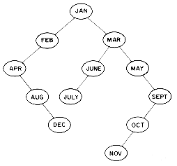
Figure 9.7 Binary search tree obtained for the months of the year.
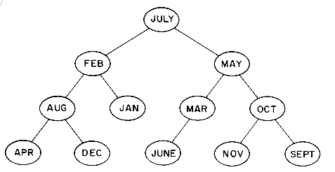
Figure 9.8 A balanced tree for the months of the year.
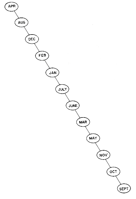
Figure 9.9 Degenerate binary search tree
Height Balanced Binary Trees
 1 where hL and hR are the heights of TL and TR respectively.
Figure 9.10 Balanced trees obtained for the months of the year.

Figure 9.10 (continued)

Figure 9.10 (continued)
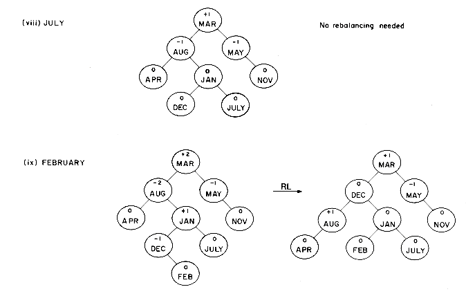
Figure 9.10 (continued)
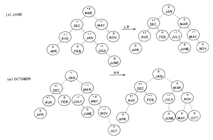
Figure 9.10 (continued)
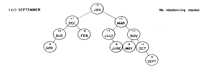
Figure 9.10 (continued)
 2. The insertion of JANUARY results in an unbalanced tree. This time, however, the rotation involved is somewhat more complex than in the earlier situations. The common point, however, is that it is still carried out with respect to the nearest parent of JANUARY with balance factor
  2. MARCH becomes the new root. AUGUST together with its left subtree becomes the left subtree of MARCH. The left subtree of MARCH becomes the right subtree of AUGUST. MAY and its right subtree, which have identifiers greater than MARCH, become the right subtree of MARCH. If MARCH had a non-empty right subtree, this could have become the left subtree of MAY since all identifiers would have been less than MAY. Inserting DECEMBER and JULY necessitates no rebalancing. When FEBRUARYis inserted the tree again becomes unbalanced. The rebalancing process is very similar to that used when JANUARY was inserted. The nearest parent with balance factor
  2 is AUGUST. DECEMBER becomes the new root of that subtree. AUGUST with its left subtree becomes the left subtree. JANUARY and its right subtree becomes the right subtree of DECEMBER, while FEBRUARY becomes the left subtree of JANUARY. If DECEMBER had had a left subtree, it would have become the right subtree of AUGUST. The insertion of JUNE requires the same rebalancing as in figure 9.10 (vi). The rebalancing following the insertion of OCTOBER is identical to that following the insertion of NOVEMBER. Inserting SEPTEMBER leaves the tree balanced.
 2. The following characterization of rotation types is obtained:
 2 as a result of the insertion. A moment's reflection will show that if a height balanced binary tree becomes unbalanced as a result of an insertion then these are the only four cases possible for rebalancing (if a moment's reflection doesn't convince you, then try exercise 6). In both the example of figure 9.10 and the rotations of figures 9.11 and 9.12, notice that the height of the subtree involved in the rotation is the same after rebalancing as it was before the insertion. This means that once the rebalancing has been carried out on the subtree in question, it is not necessary to examine the remaining tree. The only nodes whose balance factors can change are those in the subtree that is rotated.
 2. In order for a node's balance factor to become
  2, its balance factor must have been
  1 before the insertion. Furthermore, the nearest ancestor whose balance factor becomes
  2 is also the nearest ancestor with balance factor
  1 before the insertion. Therefore, before the insertion, the balance factors of all nodes on the path from A to the new insertion point must have been 0. With this information, the node A is readily determined to be the nearest ancestor of the new node having a balance factor
  1 before insertion. To complete the rotations the address of F, the parent of A, is also needed. The changes in the balance factors of the relevant nodes is shown in figures 9.11 and 9.12. Knowing F and A, all these changes can easily be carried out. What happens when the insertion of a node does not result in an unbalanced tree (figure 9.10 (i), (ii), (iv), (vii), (viii) and (xii))? While no restructuring of the tree is needed, the balance factors of several nodes change. Let A be the nearest ancestor of the new node with balance factor
  1 before insertion. If as a result of the insertion the tree did not get unbalanced even though some path length increased by 1, it must be that the new balance factor of A is 0. In case there is no ancestor A with balance factor
  1 (as in figure 9.10 (i), (ii), (iv), (vii) and (xii)), let A be the root. The balance factors of nodes from A to the parent of the new node will change to
  (see figure 9.10 (viii), A = JANUARY). Note that in both cases the procedure for determining A is the same as when rebalancing is needed. The remaining details of the insertion-rebalancing process are spelled out in algorithm AVL-INSERT.
Figure 9.11 Rebalancing rotations of type LL and RR
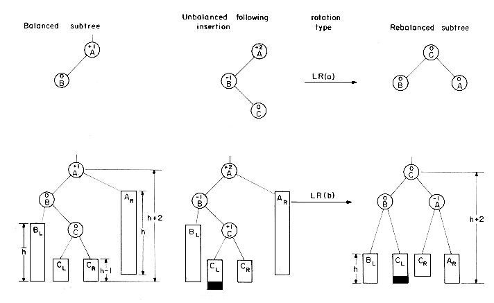
Figure 9.12 Rebalancing rotations of type LR and RL
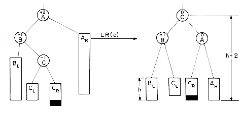
Figure 9.12 (continued)
 0. From Fibonacci number theory it is known that
  where
where  . Hence,
  . This means that if there are n nodes in the tree, then its height, h, is at most log (
 . The worst case insertion time for a height balanced tree with n nodes is, therefore, O(log n).
procedure AVL-INSERT(X,Y,T,)
//the identifier X is inserted into the AVL tree with root T. Each
node is assumed to have an identifier field IDENT, left and right
child fields LCHILD and RCHILD and a two bit balance factor
field BF. BF(P) = height of LCHILD(P) - height of RCHILD(P).
Y is set such that IDENT(Y) = X.//
//special case: empty tree T = 0.//
if T = 0 then [call GETNODE(Y); IDENT(Y)
 X; T
X; T  Y;
Y;BF(T)
 0;
0;LCHILD(T)
 0; RCHILD(T)
  0; return]
//Phase 1: Locate insertion point for X. A keeps track of most recent
node with balance factor
 1 and F is the parent of A. Q follows
P through the tree.//
F
 0; A
0; A  T; P
T; P  T; Q
T; Q  0
0while P
 0 do //search T for insertion point for X//
if BF(P)
 0 then [A
  P; F
P; F  Q]
Q]case
:X < IDENT(P): Q
 P; P
P; P  LCHILD(P) //take left
branch//
:X > IDENT(P): Q
 P; P
P; P  RCHILD(P) //take right
branch//
:else: Y
 P; return //X is in T//
end
end
//Phase 2: Insert and rebalance. X is not in T and may be inserted
as the appropriate child of Q//
call GETNODE(Y); IDENT(Y)
 X; LCHILD(Y)
  0;
0;RCHILD(Y)
 0; BF(Y)
  0
0if X < IDENT(Q) then LCHILD(Q)
 Y //insert as left child//
else RCHILD(Q)
 Y //insert as right child//
//adjust balance factors of nodes on path from A to Q. Note that
by the definition of A, all nodes on this path must have balance
factors of 0 and so will change to
 1. d = +1 implies X is inserted
in left subtree of A. d = -1 implies X is inserted in right subtree
of A//
if X > IDENT(A) then [P
 RCHILD(A); B
  P; d
P; d  -1]
-1]else [P
 LCHILD(A); B
  P; d
P; d  +1]
+1]while P
 Y do
Y doif X > IDENT(P)
then [BF(P)
 -1; P
-1; P  RCHILD(P)] //heigth of right
increases by 1//
else [BF(P)
 +1; P
+1; P  LCHILD(P)] //height of left
increases by 1//
end
//Is tree unbalanced?//
if BF(A) = 0 then [BF(A)
 d; return //tree still balanced//
if BF(A) + d = 0 then [BF(A)
 0; return //tree is balanced//
//tree unbalanced, determine rotation type//
if d = +1 then //left imbalance//
case
:BF(B) = +1; //rotation type LL//
LCHILD(A)
 RCHILD(B); RCHILD(B)
  A;
A;BF(A)
 BF(B)
BF(B)  0
0:else: //type LR//
C
 RCHILD(B)
RCHILD(B)
 LCHILD(C)
LCHILD(A)
 RCHILD(C)
LCHILD(C)
 B
BRCHILD(C)
 A
Acase
:BF(C) = +1: BF(A)
 -1; BF(B)
  0 //LR(b)//
:BF(C) = -1: BF(B)
 +1; BF(A)
  0 //LR(c)//
:else:BF(B)
 0; BF(A)
  0; //LR(a)//
end
BF(C)
 0; B
0; B  C //B is a new root//
end
else [// right imbalance; this is symmetric to left imbalance//
//and is left as an exercise//]
//subtree with root B has been rebalanced and is the new subtree//
//of F. The original subtree of F had root A
case
:F = 0 :T
 B
B:A = LCHILD(F) : LCHILD(F)
 B
B:A = RCHILD(F) : RCHILD(F)
 B
Bend
end AVL__INSERT
Operation Sequential List Linked List AVL-Tree
---------------------------------------------------------------------
Search for X O(log n) O(n) O(log n)
Search for kth item O(1) O(k) O(log n)
Delete X O(n) O(1) O(log n)
(doubly linked list
and position of X
known)
Delete kth item O(n - k) O(k) O(log n)
Insert X O(n) O(1) O(log n)
(if position for
insertion is known)
Output in order O(n) O(n) O(n)
Table 9.12 Comparison of various structures
9.3 HASH TABLES
 0
0 i
i 5 26 x 36i >1.6 x 10⁹ distinct possible values for X. Any reasonable program, however, would use far less than all of these identifiers. The ratio n / T is the identifier density, while
  = n /(sb) is the loading density or loading factor. Since the number of identifiers, n, in use is usually several orders of magnitude less than the total number of possible identifiers, T, the number of buckets b, in the hash table is also much less then T. Therefore, the hash function f must map several different identifiers into the same bucket. Two identifiers I1, I2 are said to be synonyms with respect to f if f(I1) = f(I2). Distinct synonyms are entered into the same bucket so long as all the s slots in that bucket have not been used. An overflow is said to occur when a new identifier I is mapped or hashed by f into a full bucket. A collision occurs when two nonidentical identifiers are hashed into the same bucket. When the bucket size s is 1, collisions and overflows occur simultaneously.
 , for this table is 10/52 = 0.19. The hash function f must map each of the possible identifiers into one of the numbers 1-26. If the internal binary representation for the letters A-Z corresponds to the numbers 1-26 respectively, then the function f defined by: f(X) = the first character of X; will hash all identifiers X into the hash table. The identifiers GA, D, A, G, L, A2, A1, A3, A4 and E will be hashed into buckets 7, 4, 1, 7, 12, 1, 1, 1, 1 and 5 respectively by this function. The identifiers A, A1, A2, A3 and A4 are synonyms. So also are G and GA. Figure 9.13 shows the identifiers GA, D, A, G, and A2 entered into the hash table. Note that GA and G are in the same bucket and each bucket has two slots. Similarly, the synonyms A and A2 are in the same bucket. The next identifier, A1, hashes into the bucket HT(1). This bucket is full and a search of the bucket indicates that A1 is not in the bucket. An overflow has now occurred. Where in the table should A1 be entered so that it may be retrieved when needed? We will look into overflow handling strategies in section 9.3.2. In the case where no overflows occur, the time required to enter or search for identifiers using hashing depends only on the time required to compute the hash function f and the time to search one bucket. Since the bucket size s is usually small (for internal tables s is usually 1) the search for an identifier within a bucket is carried out using sequential search. The time, then, is independent of n the number of identifiers in use. For tree tables, this time was, on the average, log n. The hash function in the above example is not very well suited for the use we have in mind because of the very large number of collisions and resulting overflows that occur. This is so because it is not unusual to find programs in which many of the variables begin with the same letter. Ideally, we would like to choose a function f which is both easy to compute and results in very few collisions. Since the ratio b/T is usually very small, it is impossible to avoid collisions altogether.
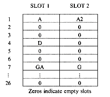
Figure 9.13 Has table with 26 buckets and two slots per bucket
9.3.1 Hashing Functions
 m, is computed by squaring the identifier and then using an appropriate number of bits from the middle of the square to obtain the bucket address; the identifier is assumed to fit into one computer word. Since the middle bits of the square will usually depend upon all of the characters in the identifier, it is expected that different identifiers would result in different hash addresses with high probability even when some of the characters are the same. Figure 9.14 shows the bit configurations resulting from squaring some sample identifiers. The number of bits to be used to obtain the bucket address depends on the table size. If r bits are used, the range of values is 2r, so the size of hash tables is chosen to be a power of 2 when this kind of scheme is used.
IDENTIFIER INTERNAL REPRESENTATION
X X X2
--------------------------------------------------
A 1 1
A1 134 20420
A2 135 20711
A3 136 21204
A4 137 21501
A9 144 23420
B 2 4
C 3 11
G 7 61
DMAX 4150130 21526443617100
DMAX1 415013034 5264473522151420
AMAX 1150130 1345423617100
AMAX1 115013034 3454246522151420
Figure 9.14 Internal representations of X and X2 in octal notation. X is input right justified, zero filled, six bits or 2 octal digits per character.
 6 the identifiers A1, B1, C1, X41, DNTXY1, etc. all have the same bucket address. With M = 2i, i
  12 the identifiers AXY, BXY, WTXY, etc. have the same bucket address. Since programmers have a tendency to use many variables with the same suffix, the choice of M as a power of 2 would result in many collisions. This choice of M would have even more disastrous results if the identifier X is stored left justified zero filled. Then, all 1 character identifiers would map to the same bucket, 0, for M = 2i, i
  54; all 2 character identifiers would map to the bucket 0 for M = 2i, i
  48 etc. As a result of this observation, we see that when the division function fD is used as a hash function, the table size should not be a power of 2 while when the "middle of square" function fm is used the table size is a power of 2. If M is divisible by 2 then odd keys are mapped to odd buckets (as the remainder is odd) and even keys are mapped to even buckets. The use of the hash table is thus biased.
Figure 9.15 Identifier Al right and left justified and zero filled. (6 bits per character)
(fD(X) - fD (Y))mod p
= (64 mod 3 C(x1)mod 3 + C(x2)mod 3
- 64 mod 3 C(x2)mod 3 - C(x1)mod 3) mod 3
= C(x1)mod 3 + C(x2)mod 3 - C(x2)mod 3 - C(x1)mod 3
= 0 mod 3.
 a where k and a are small numbers and r is the radix of the character set (in the above example r = 64), then X mod M tends to be a simple superposition of the characters in X. Thus, a good choice for M would be: M a prime number such that M does not divide rk
  a for small k and a. In section 9.3.2 we shall see other reasons for choosing M a prime number. In practice it has been observed that it is sufficient to choose M such that it has no prime divisors less than 20.
Figure 9.16 Two methods of folding
9.3.2 Overflow Handling

Figure 9.17 Hash table with linear probing. 26 buckets, 1 slot per bucket
procedure LINSRCH (X,HT,b,j)
//search the hash table HT(0: b - 1) (each bucket has exactly 1
slot) using linear probing. If HT (j = 0 then the j-th bucket is empty
and X can be entered into the table. Otherwise HT (j) = X which
is already in the table. f is the hash function//
i
 f(X); j
  i // compute hash address for X//
while HT(j)
 X and HT(j)
  0 do
0 doj
 (j + 1) mod b //treat the table as circular//
if j = i then call TABLE_FULL //no empty slots//
end
end LINSRCH
 ) / (2 - 2
 ) where
  is the loading density. This is the average over all possible sets of identifiers yielding the given loading density and using a uniform function f. In the above example
  = 12/26 = .47 and P = 1.5. Even though the average number of probes is small, the worst case can be quite large.
 i
i  b - 1 where b is the number of buckets in the table. In quadratic probing, a quadratic function of i is used as the increment. In particular, the search is carried out by examining buckets f(X), (f(X) + i2) mod b and (f(X) - i2) mod b for 1
  i
i  (b - 1)/2. When b is a prime number of the form 4j + 3, for j an integer, the quadratic search described above examines every bucket in the table. The proof that when b is of the form 4j + 3, quadratic probing examines all the buckets 0 to b - 1 relies on some results from number theory. We shall not go into the proof here. The interested reader should see Radke [1970] for a proof. Table 9.18 lists some primes of the form 4j + 3. Another possibility is to use a series of hash functions f1,f2, ...,fm. This method is known as rehashing. Buckets fi(X), 1
  i
i  m are examined in that order. An alternate method for handling bucket overflow, random probing, is discussed in exercise 19.
 Prime j Prime j
-------------------------
3 0 43 10
7 1 59 14
11 2 127 31
19 4 251 62
23 5 503 125
31 7 1019 254
Table 9.18 Some primes of the form 4j + 3
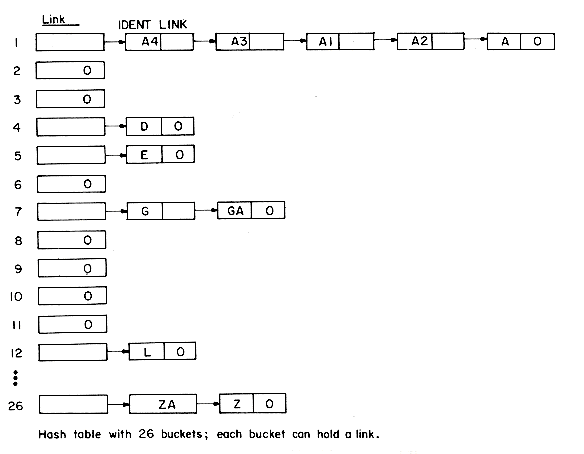
Figure 9.19. Hash chains corresponding to Figure 9.17.
procedure CHNSRCH (X,HT,b,j)
//search the hash table HT (0:b - 1) for X. Either HT(i) = 0 or it
is a pointer to the list of identifiers X: f(X) = i. List nodes have
field IDENT and LINK. Either j points to the node already containing
X or j = 0//
j
 HT (f(X)) //compute head node address//
//search the chain starting at j//
while j
 0 and IDENT (j)
  X do
X doj
 LINK (j)
end
end CHNSRCH
 where
where  is the loading density n / b (b = number of head nodes). For
  = 0.5 this figure is 1.25 and for
  = 1 it is about 1.5. This scheme has the additional advantage that only the b head nodes must be sequential and reserved at the beginning. Each head node, however, will be at most 1/2 to 1 word long. The other nodes will be much bigger and need be allocated only as needed. This could represent an overall reduction in space required for certain loading densities despite the links. If each record in the table is five words long, n = 100 and
  = 0.5, then the hash table will be of size 200 x 5 = 1000 words. Only 500 of these are used as
  = 0.5. On the other hand, if chaining is used with one full word per link, then 200 words are needed for the head nodes (b = 200). Each head node is one word long. One hundred nodes of six words each are needed for the records. The total space needed is thus 800 words, or 20% less than when no chaining was being used. Of course, when
  is close to 1, chaining uses more space than linear probing. However, when
  is close to 1, the average number of probes using linear probing or its variations becomes quite large and the additional space used for chaining can be justified by the reduction in the expected number of probes needed for retrieval. If one wishes to delete an entry from the table, then this can be done by just removing that node from its chain. The problem of deleting entries while using open addressing to resolve collisions is tackled in exercise 17.
Figure 9.20 Average number of bucket accesses per identifier retrieved (condensed from Lum, Yuen and Dodd, "Key-to-Address Transform Techniques: A Fundamental Performance Study on Large Existing Formatted Files," CACM, April 1971, Vol. 14, No. 4, pp. 228-239.)
9.3.3 THEORETICAL EVALUATION OF OVERFLOW TECHNIQUES
 i
i  n. Then, Sn is the average number of comparisons needed to find the j'th key Xj; averaged over 1
  j
j  n with each j equally likely and averaged over all bn hash sequences assuming each of these to also be equally likely. Let Un be the expected number of identifier comparisons when a search is made for an identifier not in the hash table. This hash table contains n identifiers. The quantity Un may be defined in a manner analogous to that used for Sn.
 = n/b be the loading density of a hash table using a uniform hashing function f. Then:


 1 +
1 +  /2
/2 (X)= i and chain i has k nodes on it (not including the head node) then k comparisons are needed if X is not on the chain. If X is j nodes away from the head node, 1
  j
j  k then j comparisons are needed.
 . Since, Un = expected number of identifiers on a chain, we get Un =
  .
.
REFERENCES
EXERCISES
 0.
0. 1.
1. i < j
i < j  4 for the identifier set (a1,a2,a3,a4) = (end, goto, print, stop) with p1 = 1/20, p2 = 1/5, p3= 1/10, p4= 1/20, qo= 1/5, q1 = 1/10, q2 = 1/5, q3 = 1/20, q4 = 1/20. Using the rij's construct the optimal binary search tree.
 i
i  j
j  n. Show that this can be done in time O(n).
 X and all those in T2 are > X.
 0.
0. i
i  b - 1 where S(i) is a pseudo random number. The random number generator must satisfy the property that every number from 1 to b - 1 must be generated exactly once. (i) Show that for a table of size 2r, the following sequence of computations generates numbers with this property:
 R * 5
R * 5 low order r + 2 bits of R
 R/4
R/4 )log(1 -
  ) for large table sizes.
  is the loading factor.
 | x | /2
  and | x2 | =
  | x | /2
  . Consider the following hash function
 X
X  m and that m + n units of space are available where n is the number of insertions to be made (Hint: use two arrays A(1:n) and B(1:m) where A(i) will be the ith identifier inserted into the table. If X is the ith identifier inserted then B(X) = i.). Write algorithms to search, insert and delete identifiers. Note that you cannot initialize either A or B to zero as this would take O(n + m) time. Note that X is an integer.
 xi
xi  m, 1
m, 1  i
i  n and 1
  yi m, 1
  i
i  r. Using the idea of exercise 22 write an algorithm to determine if S
  T. Your algorithm should work in O(r + n) time. since S
  T iff S
  T and T
  S, this implies that one can determine in linear time if two sets are equivalent. How much space is needed by your algorithm?
 1 we define a height balanced tree HB(k) as below:
 k where hL and hR are the heights of TL and TR respectively.


