One way to develop quicksort is to attempt a recursive solution to the problem of sorting an array data of n records. The general recursive method immediately prescribes guidelines?/FONT>break up the original problem into smaller versions of the original problem and then achieve the solution from their solutions. Here, this dictates that the original array be broken down into component arrays, which can be sorted independently and from which the final sorted array can be derived.
Thus data is to be separated into two components to be sorted, an upper array and a lower array. We then have two options for proceeding. One is to combine or merge the resultant two sorted component arrays to achieve a final sorted solution. This method is the merge sort, which is not pursued here but is applied to the sorting of files in Chapter 11. The second approach, which is taken here, is to ensure that the resultant two sorted component arrays require no further processing, but yield the final sorted solution directly.
Merely splitting data into two components and then sorting each component independently is not sufficient to guarantee that the resultant array is sorted, with no further processing required. This is because some entries in the upper component may be smaller than some entries in the lower component. For example, suppose the initial array is data, shown in Figure 8.14(a), and the upper and lower components consist, respectively, of entries 1 to 4 and 5 to 8. Sorting these components independently yields Figure 8.14(b), which is clearly not sorted.
Notice, however, that if all entries in the upper component were no less than all entries in the lower component, then sorting each component independently would always lead to a result that is sorted. For example, suppose the initial array is Figure 8.14(c). Taking the upper and lower components as entries 1 to 4, and 5 to 8, respectively, and independently sorting them produces Figure 8.14(d). This array is now sorted.
Note that the fifth entry, 13, occupies the same position in the sorted array as in the initial array. This is because all entries in the upper component are no less, and all entries in the lower component are no greater, than 13. The key value 13 actually occupied its proper position in the sorted version of data before the two components were sorted. Hence it need not be included in either component and may serve as a separator or partitioning entry between the two components to be sorted.
To carry out this procedure for an arbitrary array requires finding a partitioning entry. Normally a partitioning entry, such as 13 in position 5, will not occur in the initial array to be sorted. For example, no such partitioning entry (separating larger entries above from smaller entries below) occurs in Figure 8.14(a). This means that the initial array must be rearranged so that a partitioning entry may be found and subsequently used to separate the components.
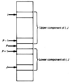
In keeping with the top-down approach, assume that this task (rearranging the initial array and determining a partitioning entry) is carried out by the function partition(i,j). The arguments i and j contain pointers to entries of the array, as shown in Figure 8.15. Partition (i,j) returns an index pointer to a partitioning entry of the array consisting of all entries between i and j. Thus, if partition (i,j) returns a value p, then all entries between i and p? are at least as great as data [p].key, and all entries between p+1 and j are no greater than data [p].key. The pointer p separates the upper and lower components of i,j.
8.5.1 Two Quicksort Procedures
8.5.3 Analyzing Iterative Quicksort
8.5.4 The Worst and Best Cases
8.5.5 Distributive Partitioning

Figure 8.14 Sorting an Array by Component

Figure 8.15 Array with a Partitioning Entry P Separating Upper and Lower Components