12.4.1 Finding Optimal Binary Search Trees

An obvious way to find an optimal binary search tree is to generate each possible binary search tree for the keys, calculate its weighted path length, and keep that tree with the smallest weighted path length. This search through all possible solutions is not feasible except for small n, since the number of such trees grows exponentially with n. A feasible alternative would be a recursive algorithm based on the structure inherent in optimal binary search trees. Such an algorithm can be developed in a way similar to that used for the construction of Fibonacci trees in Chapter 7.

How do we decompose the optimal search tree problem in Example 12.2 into components with the same structure? Consider the characteristics of any optimal tree. Of course, it has a root and two subtrees. A moment's reflection should convince you that both subtrees must themselves be optimal binary search trees with respect to their keys and weights. First, any subtree of any binary search tree must be a binary search tree. Second, the subtrees must also be optimal. Otherwise, they could be replaced by optimal subtrees with smaller weighted path lengths, which would imply that the original tree could not have been optimal.

Since there are n possible keys as candidates for the root of the optimal tree, the recursive solution must try them all. For each candidate key as root, all keys less than that key must appear in its left subtree, and all keys greater than it must appear in its right subtree. To state the recursive algorithm based on these observations requires some notation.

Denote the weights assigned to the n stored keys by b's and the weights assigned to the terminal nodes by a's. The weight assigned to k_i is b_i for i = 1, 2, . . . , n, and that assigned to the external node labeled i is ai for i = 0, 1, 2, . . . , n. Let obst(i,j) denote the optimal binary search tree containing keys k_i, . . . , k_j, and let w(i,j) denote its weighted path length. Obst(i,j) will involve weights a_i-1, b_i, . . . , b_i, a_j.

The optimal tree with root constrained to be k_k and containing keys k_i, . . . , k_k, . . . , k_j must then have obst(i,k-1) as its left subtree and obst(k+1,...,j) as its right subtree. Its weighted path length, w(i, j), is given by sw(i, j) + w(i, k - 1) + w(k + 1, j), where sw(i, j) is the sum of the weights a_i-1, b_i, . . . , b_j, a_j. Sw(i, j) is the value assigned to the root of obst(i,j), the sum of its weights.

Finally the algorithm can be stated.

For each k(k) as root, k = 1, 2, . . . , n

find obst(1,k-1) and obst(k+1,n).

Find a k that minimizes [w(1, k - 1) + w(k + 1, n)] over k = 1, 2, . . . , n.

Obst(1,n) is given by the tree with root k_k, obst(1,k-1) as its left subtree, and

obst(k+1,n) as its right subtree.

The weighted path length of obst(1,n) is w(1, n).

w(1, n) = sw(1, n) + w(1, k-1) + w(k+1, n).

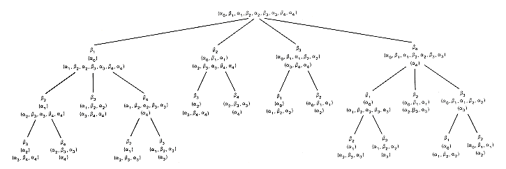
The execution tree for obst(1,4) is given in Figure 12.10. Apparently this algorithm exhibits the same proliferation of recursive calls for identical component problems as did the algorithm for the Fibonacci tree construction in Chapter 7. These are summarized in Table 12.1. This inefficiency can be avoided by using a bottom-up construction, just as was done for Fibonacci trees. To do this requires a clear understanding of exactly which optimal subtrees must be retained for later reference.

All possible optimal subtrees are not required. Those that are needed consist of sequences of keys that are immediate successors of the smallest key in the

Table 12.1 Components Replicated by Recursive Calls

Replicated Component  Occurrences

----------------------------------

 (a2, b3, a3, b4, a4)       2

 (a0, b1, a1, b2, a2)       2

 (a1, b2, a2, b3, a3)       2

 (a0, b1, a1)               4

 (a1, b2, a2)               5

 (a2, b3, a3)               5

 (a3, b4, a4)               4

 (a0)                       4

 (a1)                       3

 (a2)                       4

 (a3)                       3

 (a4)                       4

Figure 12.10 The Execution Tree for n = 4

subtree, successors in the sorted order for the keys. The final solution tree contains all n keys. There will be two with n - 1 keys, three with n - 2 keys, four with n - 3 keys, and in general k + 1 with n - k keys, for k = 0, 1, 2, . . . , n. Consequently there are a total of (n + 1) ?/FONT> (n + 2)/2 optimal subtrees to be retained. Notice that to determine obst(i,j) requires knowing the optimal smaller subtrees involving weights:

(ai?SUB>1) and (ai, bi+1, . . . , bj, aj)

i.e., obst(i,i?) and obst(i+1,j)

(ai-1, bi, ai) and (ai+1, bi+2, . . . , Bj, aj)

i.e., obst(i,i) and obst(i+2,j)

(ai-1, bi, . . . , bj-1, aj-1) and (aj)

i.e., obst(i,j-1) and obst(j+1,j)

The bottom-up approach generates all smallest required optimal subtrees first, then all next smallest, and so on until the final solution involving all the weights is found. Since the algorithm requires access to each subtree's weighted path length, these weighted path lengths must also be retained to avoid their recalculation. Finally, the root of each subtree must also be stored for reference.

This algorithm requires O(n³) execution time and O(n²) storage. Knuth, who developed this solution, noticed an important fact that reduces the execution time to O(n²). He was able to show that the minimization need not be over all k from 1 to n. Instead, the minimization may be taken only over all k between r(i,j - 1) and r(i + 1,j), where r(i,j) denotes the root of obst(i,j). See Knuth [1973b].

Intuitively, this is plausible because obst(i,j-1) is the optimal binary search tree containing keys k_i, . . . , k_r(i,j-1), . . . , k_j-1. Thus taking k_r(i,j-1) as its root gives the tree just the "balance" it needs to be optimal, distributing keys to its left and right subtrees in the optimal way. Obst(i,j) includes k_j as well. If its root is also k_r(i,j-1), then k_j will appear in the right subtree of this optimal tree adding more weight to its right subtree. Think of the optimal tree as "balanced." Its root should not be a predecessor of k_r(i,j-1), since this would cause even more weight to appear in its right subtree. Reasoning this way, it is not unreasonable to expect the root of obst(i,j) to be k_r(i,j-1) or one of its successors. Thus looking only at k where r(i, j - 1) ?/FONT> k should suffice. A symmetrical argument should make it equally reasonable that looking only at k, k ?/FONT> r(i + 1, j) should suffice. The actual proof is complex and adds little insight, so it is omitted here.

The bottom-up algorithm, incorporating the new minimization limits, may now be written.

1. For i from 0 to n

a. Set w(i + 1, i) to 0 and sw(i + 1, i) to a_i

b. For j from i + 1 to n

Set sw(i + 1, j) to sw(i + 1, j - 1) + b_j + a_j

2. For j from 1 to n

a. Set w(j, j) to sw(j, j) and r(j, j) to j.

(This initializes all obst's containing 0 keys and 1 key.)

3. For l from 2 to n

a. For j from l to n,

i. set i to j - l + 1;

ii set w(i, j) to sw(i, j) + minimum[w(i, k - 1) + w(k + 1,j)], the minimum to be over k satisfying r(i, j - 1) ?/FONT> k ?/FONT> r(i + 1, j) and set r(i, j) to a value of k corresponding to the minimum.

Actually, the w(i,j)'s will differ from the weighted path length of obst(i,j) by the sum of a_i-1, a_i, . . . , a_j. This does not affect the final tree but means that to obtain the true weighted path length, a₀ + a₁ + . . . + a_n must be added to w(1, n).

Arrays for w, ws, and r seem to be a natural choice for implementing this algorithm and provide rapid access to the information required for the processing involved.

Example 12.3

Find the optimal binary search tree for n = 6 and weights b₁= 10, b₂= 3, b₃= 9, b₄= 2, b₅= 0, b₆= 10, a₀= 5, a₁= 6, a₂= 4, a₃= 4, a₄= 3, a₅= 8, a₆= 0. n

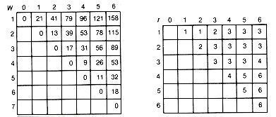
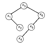
Figure 12.11(a) shows the arrays as they would appear after the initialization, and 12.11(b) gives their final disposition. The actual optimal tree is shown in Figure 12.12. It has a weighted path length of 188.

Since this algorithm requires O(n² ) time and O(n²) storage, as n increases, it will run out of storage even before it runs out of time. The storage needed can be reduced by almost half, at the expense of a slight increase in time, by implementing the two-dimensional arrays as one-dimensional arrays using the technique of Chapter 2. Using one-dimensional arrays may enable problems to be solved that otherwise will abort because of insufficient storage. In any case, the algorithm is feasible only for moderate values of n.

(a) Initial Array Values

(b) Final Array Values

Figure 12.11 Arrays Used to Implement the Bottom-up Recursive Algorithm for Finding Optimal Binary Search Trees

Figure 12.12 The Optimal Binary Search Tree Found by Means of the Bottom-up Recursive Algorithm

In order to understand exactly how the algorithm creates the optimal tree, you should simulate the algorithm to reproduce the arrays of Figure 12.11.