


As noted in Chapter 1, when an algorithm contains a recursive call to itself, its running time can often be described by a recurrence. A recurrence is an equation or inequality that describes a function in terms of its value on smaller inputs. For example, we saw in Chapter 1 that the worst-case running time T(n) of the MERGE-SORT procedure could be described by the recurrence
whose solution was claimed to be T(n) =
This chapter offers three methods for solving recurrences--that is, for obtaining asymptotic "
where a
In practice, we neglect certain technical details when we state and solve recurrences. A good example of a detail that is often glossed over is the assumption of integer arguments to functions. Normally, the running time T(n) of an algorithm is only defined when n is an integer, since for most algorithms, the size of the input is always an integer. For example, the recurrence describing the worst-case running time of MERGE-SORT is really
Boundary conditions represent another class of details that we typically ignore. Since the running time of an algorithm on a constant-sized input is a constant, the recurrences that arise from the running times of algorithms generally have T(n) =
without explicitly giving values for small n. The reason is that although changing the value of T(1) changes the solution to the recurrence, the solution typically doesn't change by more than a constant factor, so the order of growth is unchanged.
When we state and solve recurrences, we often omit floors, ceilings, and boundary conditions. We forge ahead without these details and later determine whether or not they matter. They usually don't, but it is important to know when they do. Experience helps, and so do some theorems stating that these details don't affect the asymptotic bounds of many recurrences encountered in the analysis of algorithms (see Theorem 4.1 and Problem 4-5). In this chapter, however, we shall address some of these details to show the fine points of recurrence solution methods.
The substitution method for solving recurrences involves guessing the form of the solution and then using mathematical induction to find the constants and show that the solution works. The name comes from the substitution of the guessed answer for the function when the inductive hypothesis is applied to smaller values. This method is powerful, but it obviously can be applied only in cases when it is easy to guess the form of the answer.
The substitution method can be used to establish either upper or lower bounds on a recurrence. As an example, let us determine an upper bound on the recurrence
which is similar to recurrences (4.2) and (4.3). We guess that the solution is T(n) = O(n lg n). Our method is to prove that T(n)
where the last step holds as long as c
Mathematical induction now requires us to show that our solution holds for the boundary conditions. That is, we must show that we can choose the constant c large enough so that the bound T(n)
This difficulty in proving an inductive hypothesis for a specific boundary condition can be easily overcome. We take advantage of the fact that asymptotic notation only requires us to prove T(n)
Unfortunately, there is no general way to guess the correct solutions to recurrences. Guessing a solution takes experience and, occasionally, creativity. Fortunately, though, there are some heuristics that can help you become a good guesser.
If a recurrence is similar to one you have seen before, then guessing a similar solution is reasonable. As an example, consider the recurrence
which looks difficult because of the added "17" in the argument to T on the right-hand side. Intuitively, however, this additional term cannot substantially affect the solution to the recurrence. When n is large, the difference between T(
Another way to make a good guess is to prove loose upper and lower bounds on the recurrence and then reduce the range of uncertainty. For example, we might start with a lower bound of T(n) =
There are times when you can correctly guess at an asymptotic bound on the solution of a recurrence, but somehow the math doesn't seem to work out in the induction. Usually, the problem is that the inductive assumption isn't strong enough to prove the detailed bound. When you hit such a snag, revising the guess by subtracting a lower-order term often permits the math to go through.
Consider the recurrence
We guess that the solution is O(n), and we try to show that T(n)
which does not imply T(n)
Intuitively, our guess is nearly right: we're only off by the constant 1, a lower-order term. Nevertheless, mathematical induction doesn't work unless we prove the exact form of the inductive hypothesis. We overcome our difficulty by subtracting a lower-order term from our previous guess. Our new guess is T(n)
as long as b
Most people find the idea of subtracting a lower-order term counterintuitive. After all, if the math doesn't work out, shouldn't we be increasing our guess? The key to understanding this step is to remember that we are using mathematical induction: we can prove something stronger for a given value by assuming something stronger for smaller values.
It is easy to err in the use of asymptotic notation. For example, in the recurrence (4.4) we can falsely prove T(n) = O(n) by guessing T(n)
since c is a constant. The error is that we haven't proved the exact form of the inductive hypothesis, that is, that T(n)
Sometimes, a little algebraic manipulation can make an unknown recurrence similar to one you have seen before. As an example, consider the recurrence
which looks difficult. We can simplify this recurrence, though, with a change of variables. For convenience, we shall not worry about rounding off values, such as
We can now rename S(m) = T(2m) to produce the new recurrence
which is very much like recurrence (4.4) and has the same solution: S(m) = O(m lg m). Changing back from S(m) to T(n), we obtain T(n) = T(2m) = S(m) = O(m lg m) = O(lg n lg lg n).
4.1-1
Show that the solution of T(n) = T(
4.1-2
Show that the solution of T(n) = 2T(
4.1-3
Show that by making a different inductive hypothesis, we can overcome the difficulty with the boundary condition T(1) = 1 for the recurrence (4.4) without adjusting the boundary conditions for the inductive proof.
4.1-4
Show that
4.1-5
Show that the solution to T(n) = 2T(
4.1-6
Solve the recurrence
The method of iterating a recurrence doesn't require us to guess the answer, but it may require more algebra than the substitution method. The idea is to expand (iterate) the recurrence and express it as a summation of terms dependent only on n and the initial conditions. Techniques for evaluating summations can then be used to provide bounds on the solution.
As an example, consider the recurrence
We iterate it as follows:
where
How far must we iterate the recurrence before we reach a boundary condition? The ith term in the series is 3i
Here, we have used the identity (2.9) to conclude that 3log4 n = nlog43, and we have used the fact that log4 3 < 1 to conclude that
The iteration method usually leads to lots of algebra, and keeping everything straight can be a challenge. The key is to focus on two parameters: the number of times the recurrence needs to be iterated to reach the boundary condition, and the sum of the terms arising from each level of the iteration process. Sometimes, in the process of iterating a recurrence, you can guess the solution without working out all the math. Then, the iteration can be abandoned in favor of the substitution method, which usually requires less algebra.
When a recurrence contains floor and ceiling functions, the math can become especially complicated. Often, it helps to assume that the recurrence is defined only on exact powers of a number. In our example, if we had assumed that n = 4k for some integer k, the floor functions could have been conveniently omitted. Unfortunately, proving the bound T(n) = O(n) solely for exact powers of 4 is technically an abuse of the O-notation. The definitions of asymptotic notation require that bounds be proved for all sufficiently large integers, not just those that are powers of 4. We shall see in Section 4.3 that for a large class of recurrences, this technicality can be overcome. Problem 4-5 also gives conditions under which an analysis for exact powers of an integer can be extended to all integers.
Recursion trees
Exercises
The master method provides a "cookbook" method for solving recurrences of the form
where a
The recurrence (4.5) describes the running time of an algorithm that divides a problem of size n into a subproblems, each of size n/b, where a and b are positive constants. The a subproblems are solved recursively, each in time T(n/b). The cost of dividing the problem and combining the results of the subproblems is described by the function â(n). (That is, using the notation from Section 1.3.2, â(n) = D(n) + C(n).) For example, the recurrence arising from the MERGE-SORT procedure has a = 2, b = 2, and â(n) =
As a matter of technical correctness, the recurrence isn't actually well defined because n/b might not be an integer. Replacing each of the a terms T(n/b) with either T(
The master method depends on the following theorem.
Theorem 4.1
Let a
where we interpret n/b to mean either
1. If â(n) = O(nlogba-
2. If â(n) =
3. If â(n) =
Before applying the master theorem to some examples, let's spend a moment trying to understand what it says. In each of the three cases, we are comparing the function â(n) with the function nlogba. Intuitively, the solution to the recurrence is determined by the larger of the two functions. If, as in case 1, the function nlogba is the larger, then the solution is T(n) =
Beyond this intuition, there are some technicalities that must be understood. In the first case, not only must â(n) be smaller than nlogba, it must be polynomially smaller. That is, â(n) must be asymptotically smaller than nlogba by a factor of n
It is important to realize that the three cases do not cover all the possibilities for â(n). There is a gap between cases 1 and 2 when â(n) is smaller than nlogba but not polynomially smaller. Similarly, there is a gap between cases 2 and 3 when â(n) is larger than nlogba but not polynomially larger. If the function â(n) falls into one of these gaps, or if the regularity condition in case 3 fails to hold, the master method cannot be used to solve the recurrence.
To use the master method, we simply determine which case (if any) of the master theorem applies and write down the answer.
As a first example, consider
For this recurrence, we have a = 9, b = 3, â(n) = n, and thus nlogba = nlog39 =
Now consider
in which a = 1, b = 3/2, â(n) = 1, and nlogba = nlog3/21 = n0 = 1. Case 2 applies, since â(n) =
For the recurrence
we have a = 3, b = 4, â(n) = n lg n, and nlogba = nlog43 = 0(n0.793). Since â(n) =
The master method does not apply to the recurrence
even though it has the proper form: a = 2, b = 2, â(n) = n1g n, and nlogba = n. It seems that case 3 should apply, since â(n) = n1g n is asymptotically larger than nlogba = n but not polynomially larger. The ratio â(n)/nlogba = (n 1g n)/n = 1g n is asymptotically less than n
4.3-1
Use the master method to give tight asymptotic bounds for the following recurrences.
a. T(n) = 4T(n/2) + n.
b. T(n) = 4T(n/2) + n2.
c. T(n) = 4T(n/2) + n3.
4.3-2
The running time of an algorithm A is described by the recurrence T(n) = 7T(n/2) + n2. A competing algorithm A' has a running time of T'(n) = aT'(n/4) + n2. What is the largest integer value for a such that A' is asymptotically faster than A?
4.3-3
Use the master method to show that the solution to the recurrence T(n) = T(n/2) +
4.3-4
Consider the regularity condition aâ(n/b)
This section contains a proof of the master theorem (Theorem 4.1) for more advanced readers. The proof need not be understood in order to apply the theorem.
The proof is in two parts. The first part analyzes the "master" recurrence (4.5), under the simplifying assumption that T(n) is defined only on exact powers of b > 1, that is, for n = 1, b, b2, . . .. This part gives all the intuition needed to understand why the master theorem is true. The second part shows how the analysis can be extended to all positive integers n and is merely mathematical technique applied to the problem of handling floors and ceilings.
In this section, we shall sometimes abuse our asymptotic notation slightly by using it to describe the behavior of functions that are only defined over exact powers of b. Recall that the definitions of asymptotic notations require that bounds be proved for all sufficiently large numbers, not just those that are powers of b. Since we could make new asymptotic notations that apply to the set {bi : i = 0,1, . . .}, instead of the nonnegative integers, this abuse is minor.
Nevertheless, we must always be on guard when we are using asymptotic notation over a limited domain so that we do not draw improper conclusions. For example, proving that T(n) = O(n) when n is an exact power of 2 does not guarantee that T(n) = O(n). The function T(n) could be defined as
in which case the best upper bound that can be proved is T(n) = O(n2). Because of this sort of drastic consequence, we shall never use asymptotic notation over a limited domain without making it absolutely clear from the context that we are doing so.
The first part of the proof of the master theorem analyzes the master recurrence (4.5),
under the assumption that n is an exact power of b > 1, where b need not be an integer. The analysis is broken into three lemmas. The first reduces the problem of solving the master recurrence to the problem of evaluating an expression that contains a summation. The second determines bounds on this summation. The third lemma puts the first two together to prove a version of the master theorem for the case in which n is an exact power of b.
Lemma 4.2
Let a
where i is a positive integer. Then
Proof Iterating the recurrence yields
Since alogb n = nlogba, the last term of this expression becomes
using the boundary condition T(1) =
thus,
which completes the proof.
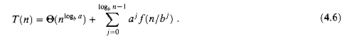
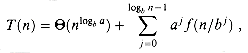
Before proceeding, let's try to develop some intuition by using a recursion tree. Figure 4.3 shows the tree corresponding to the iteration of the recurrence in Lemma 4.2. The root of the tree has cost â(n), and it has a children, each with cost â(n/b). (It is convenient to think of a as being an integer, especially when visualizing the recursion tree, but the mathematics does not require it.) Each of these children has a children with cost â(n/b2), and thus there are a2 nodes that are distance 2 from the root. In general, there are a2 nodes that are distance j from the root, and each has cost â(n/bj). The cost of each leaf is T(1) =
We can obtain equation (4.6) by summing the costs of each level of the tree, as shown in the figure. The cost for a level j of internal nodes is ajâ(n/bj), and so the total of all internal node levels is
In the underlying divide-and-conquer algorithm, this sum represents the costs of dividing problems into subproblems and then recombining the subproblems. The cost of all the leaves, which is the cost of doing all nlogba subproblems of size 1, is
In terms of the recursion tree, the three cases of the master theorem correspond to cases in which the total cost of the tree is (1) dominated by the costs in the leaves, (2) evenly distributed across the levels of the tree, or (3) dominated by the cost of the root.
The summation in equation (4.6) describes the cost of the dividing and combining steps in the underlying divide-and-conquer algorithm. The next lemma provides asymptotic bounds on the summation's growth.
Lemma 4.3
Let a
can then be bounded asymptotically for exact powers of b as follows.
1. If â(n) = O(nlogba-
2. If â(n) =
3. If aâ(n/b)
Proof For case 1, we have â(n) = O(nlogba-
We bound the summation within the O-notation by factoring out terms and simplifying, which leaves an increasing geometric series:
Since b and
and case 1 is proved.
Under the assumption that â(n) =
We bound the summation within the
Substituting this expression for the summation in equation (4.9) yields
and case 2 is proved.
Case 3 is proved similarly. Since
since c is constant. Thus, we can conclude that g(n) =
We can now prove a version of the master theorem for the case in which n is an exact power of b.
Lemma 4.4
Let a
where i is a positive integer. Then T(n) can be bounded asymptotically for exact powers of b as follows.
1. If
2. If
3. If
Proof We use the bounds in Lemma 4.3 to evaluate the summation (4.6) from Lemma 4.2. For case 1, we have
and for case 2,
For case 3, the condition a
To complete the proof of the master theorem, we must now extend our analysis to the situation in which floors and ceilings are used in the master recurrence, so that the recurrence is defined for all integers, not just exact powers of b. Obtaining a lower bound on
and an upper bound on
is routine, since the bound
We wish to iterate the recurrence (4.10), as was done in Lemma 4.2. As we iterate the recurrence, we obtain a sequence of recursive invocations on the arguments
Let us denote the ith element in the sequence by ni, where
Our first goal is to determine the number of iterations k such that nk is a constant. Using the inequality
In general,
and thus, when i =
We can now iterate recurrence (4.10), obtaining
which is much the same as equation (4.6), except that n is an arbitrary integer and not restricted to be an exact power of b.
We can now evaluate the summation
from (4.13) in a manner analogous to the proof of Lemma 4.3. Beginning with case 3, if af(
since c(1 + b/(b - 1))logba is a constant. Thus, case 2 is proved. The proof of case 1 is almost identical. The key is to prove the bound f(nj) = O(nlogba-
We have now proved the upper bounds in the master theorem for all integers n. The proof of the lower bounds is similar.
4.4-1
Give a simple and exact expression for ni in equation (4.12) for the case in which b is a positive integer instead of an arbitrary real number.
4.4-2
Show that if f(n) =
4.4-3
Show that case 3 of the master theorem is overstated, in the sense that the regularity condition af(n/b)
4-1 Recurrence examples
Give asymptotic upper and lower bounds for T(n) in each of the following recurrences. Assume that T(n) is constant for n
a. T(n) = 2T
b. T(n) = T(9n/10) + n.
c. T(n) = 16T(n/4) + n2.
d. T(n) = 7T(n/3) + n2.
e. T(n) = 7T(n/2) + n2.
g. T(n) = T(n - 1) + n.
4-2 Finding the missing integer
An array A[1 . . n] contains all the integers from 0 to n except one. It would be easy to determine the missing integer in O(n) time by using an auxiliary array B[0 . . n] to record which numbers appear in A. In this problem, however, we cannot access an entire integer in A with a single operation. The elements of A are represented in binary, and the only operation we can use to access them is "fetch the jth bit of A[i]," which takes constant time.
Show that if we use only this operation, we can still determine the missing integer in O(n) time.
4-3 Parameter-passing costs
Throughout this book, we assume that parameter passing during procedure calls takes constant time, even if an N-element array is being passed. This assumption is valid in most systems because a pointer to the array is passed, not the array itself. This problem examines the implications of three parameter-passing strategies:
1. An array is passed by pointer. Time =
2. An array is passed by copying. Time =
3. An array is passed by copying only the subrange that might be accessed by the called procedure. Time =
a. Consider the recursive binary search algorithm for finding a number in a sorted array (see Exercise 1.3-5). Give recurrences for the worst-case running times of binary search when arrays are passed using each of the three methods above, and give good upper bounds on the solutions of the recurrences. Let N be the size of the original problem and n be the size of a subproblem.
b. Redo part (a) for the MERGE-SORT algorithm from Section 1.3.1.
4-4 More recurrence examples
Give asymptotic upper and lower bounds for T(n) in each of the following recurrences. Assume that T(n) is constant for n
a. T(n) = 3T(n/2) + n 1g n.
b. T(n) = 3T(n/3 + 5) + n / 2.
c. T(n) = 2T(n/2) + n / lg n.
d. T(n) = T(n - 1) + 1 / n.
e. T(n) = T(n - 1) + 1g n.
4-5 Sloppiness conditions
Often, we are able to bound a recurrence T(n) at exact powers of an integral constant b. This problem gives sufficient conditions for us to extend the bound to all real n > 0.
a. Let T(n) and h(n) be monotonically increasing functions, and suppose that T(n) < h(n) when n is an exact power of a constant b > 1. Moreover, suppose that h(n) is "slowly growing" in the sense that h(n) = O(h(n/b)). Prove that T(n) = O(h(n)).
b. Suppose that we have the recurrence T(n) = aT(n/b) + f(n), where a
c. Simplify the proof of the master theorem for the case in which f(n) is monotonically increasing and slowly growing. Use Lemma 4.4.
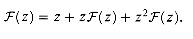
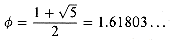
4-6 Fibonacci numbers
This problem develops properties of the Fibonacci numbers, which are defined by recurrence (2.13). We shall use the technique of generating functions to solve the Fibonacci recurrence. Define the generating function (or formal power series)
a. Show that
b. Show that
where
and
c. Show that
d. Prove that
e. Prove that Fi + 2
4-7 VLSI chip testing
Professor Diogenes has n supposedly identical VLSI1 chips that in principle are capable of testing each other. The professor's test jig accommodates two chips at a time. When the jig is loaded, each chip tests the other and reports whether it is good or bad. A good chip always reports accurately whether the other chip is good or bad, but the answer of a bad chip cannot be trusted. Thus, the four possible outcomes of a test are as follows:
1 VLSI stands for "very-large-scale integration," which is the integrated-circuit chip technology used to fabricate most microprocessors today.
a. Show that if more than n/2 chips are bad, the professor cannot necessarily determine which chips are good using any strategy based on this kind of pairwise test. Assume that the bad chips can conspire to fool the professor.
b. Consider the problem of finding a single good chip from among n chips, assuming that more than n/2 of the chips are good. Show that
c. Show that the good chips can be identified with
Recurrences were studied as early as 1202 by L. Fibonacci, for whom the Fibonacci numbers are named. A. De Moivre introduced the method of generating functions (see Problem 4-6) for solving recurrences. The master method is adapted from Bentley, Haken, and Saxe [26], which provides the extended method justified by Exercise 4.4-2. Knuth [121] and Liu [140] show how to solve linear recurrences using the method of generating functions. Purdom and Brown [164] contains an extended discussion of recurrence solving.

(4.1)
 (n lg n)." or "O" bounds on the solution. In the substitution method, we guess a bound and then use mathematical induction to prove our guess correct. The iteration method converts the recurrence into a summation and then relies on techniques for bounding summations to solve the recurrence. The master method provides bounds for recurrences of the form
T(n) = aT(n/b) +
 (n),
(n), 1, b > 1, and (n) is a given function; it requires memorization of three cases, but once you do that, determining asymptotic bounds for many simple recurrences is easy.
Technicalities

(4.2)
(1) for sufficiently small n. Consequently, for convenience, we shall generally omit statements of the boundary conditions of recurrences and assume that T(n) is constant for small n. For example, we normally state recurrence (4.1) asT(n) = 2T(n/2) +
(n),(4.3)
4.1 The substitution method
T(n) = 2T(
 n/2
n/2 ) + n,
(4.4)
 cn lg n for an appropriate choice of the constant c > 0. We start by assuming that this bound holds for n/2, that is, that T(n/2) c n/2 1g (n/2). Substituting into the recurrence yields
T(n)
2(c n/2 1g (n/2)) + n cn lg(n/2) + n= cn lg n - cn lg 2 + n
= cn lg n - cn + n
cn lg n, 1. cn lg n works for the boundary conditions as well. This requirement can sometimes lead to problems. Let us assume, for the sake of argument, that T(1) = 1 is the sole boundary condition of the recurrence. Then, unfortunately, we can't choose c large enough, since T(1) c1 lg 1 = 0. cn lg n for n n0, where n0 is a constant. The idea is to remove the difficult boundary condition T(1) = 1 from consideration in the inductive proof and to include n = 2 and n = 3 as part of the boundary conditions for the proof. We can impose T(2) and T(3) as boundary conditions for the inductive proof because for n > 3, the recurrence does not depend directly on T(1). From the recurrence, we derive T(2) = 4 and T(3) = 5. The inductive proof that T(n) cn lg n for some constant c 2 can now be completed by choosing c large enough so that T(2) c2 lg 2 and T(3) c3 lg 3. As it turns out, any choice of c 2 suffices. For most of the recurrences we shall examine, it is straightforward to extend boundary conditions to make the inductive assumption work for small n.Making a good guess
T(n) = 2T(
n/2 + 17) + n,n/2) and T(n/2 + 17) is not that large: both cut n nearly evenly in half. Consequently, we make the guess that T(n) = O(n lg n), which you can verify as correct by using the substitution method (see Exercise 4.1-5). (n) for the recurrence (4.4), since we have the term n in the recurrence, and we can prove an initial upper bound of T(n) = O(n2). Then, we can gradually lower the upper bound and raise the lower bound until we converge on the correct, asymptotically tight solution of T(n) = (n lg n).
Subtleties
T(n) = T(
n/2) + T ( n/2
n/2 ) + 1. cn for an appropriate choice of the constant c. Substituting our guess in the recurrence, we obtain
T(n)
c n/2 + c n/2 + 1= cn + 1,
cn for any choice of c. It's tempting to try a larger guess, say T(n) = O(n2), which can be made to work, but in fact, our guess that the solution is T(n) = O(n) is correct. In order to show this, however, we must make a stronger inductive hypothesis. cn - b, where b 0 is constant. We now haveT(n)
(cn/2 - b) + (cn/2 - b) + 1= cn - 2b + 1
cn - b , 1. As before, the constant c must be chosen large enough to handle the boundary conditions.Avoiding pitfalls
cn and then arguingT(n)
2(cn/2) + n cn + n= O(n),
 wrong!! cn.
Changing variables
 , to be integers. Renaming m = 1g n yields
T(2m) = 2T(2m/2) + m.
S(m) = 2S(m/2) + m,
Exercises
n/2) + 1 is O(lg n).n/2) + n is (n lg n). Conclude that the solution is (n lg n).(n lg n) is the solution to the "exact" recurrence (4.2) for merge sort.n/2 + 17) + n is O(n lg n). by making a change of variables. Do not worry about whether values are integral.
4.2 The iteration method
T(n) = 3T(
n/4) + n.T(n) = n + 3T(
n/4)= n + 3 (
n/4 + 3T(n/16))= n + 3(
n/4 + 3(n/16 + 3T(n/64)))= n + 3
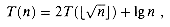
n/4 + 9 n/16 + 27T(n/64),n/4/4 = n/16 and n/16/4 = n/64 follow from the identity (2.4).n/4i. The iteration hits n = 1 when n/4i = 1 or, equivalently, when i exceeds log4 n. By continuing the iteration until this point and using the bound n/4i n/4i, we discover that the summation contains a decreasing geometric series: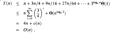 (nlog43) = o(n).
4.3 The master method
T(n) = aT(n/b)+â(n),
(4.5)
1 and b > 1 are constants and â(n) is an asymptotically positive function. The master method requires memorization of three cases, but then the solution of many recurrences can be determined quite easily, often without pencil and paper.(n).n/b) or T(n/b) doesn't affect the asymptotic behavior of the recurrence, however. (We'll prove this in the next section.) We normally find it convenient, therefore, to omit the floor and ceiling functions when writing divide-and-conquer recurrences of this form.The master theorem
1 and b > 1 be constants, let â(n) be a function, and let T(n) be defined on the nonnegative integers by the recurrenceT(n) = aT(n/b) + â(n),
n/b or n/b. Then T(n) can be bounded asymptotically as follows. ) for some constant > 0, then T(n) = (nlogba).(nlogba), then T(n) = (nlogbalg n).(nlogba+) for some constant > 0, and if aâ(n/b) câ(n) for some constant c < 1 and all sufficiently large n, then T(n) = (â(n)). (â(nlogba). If, as in case 3, the function â(n) is the larger, then the solution is T(n) = (â(n)). If, as in case 2, the two functions are the same size, we multiply by a logarithmic factor, and the solution is T(n) = (nlogba lg n) = (â(n)lg n). for some constant > 0. In the third case, not only must â(n) be larger than nlogba, it must be polynomially larger and in addition satisfy the "regularity" condition that aâ(n/b) câ(n). This condition is satisfied by most of the polynomially bounded functions that we shall encounter.
Using the master method
T(n) = 9T(n/3) + n.
(n2). Since â(n) = 0(nlog39-), where = 1, we can apply case 1 of the master theorem and conclude that the solution is T(n) = (n2).T(n) = T(2n/3) + 1,
(nlogba) = (1), and thus the solution to the recurrence is T(n) = (lg n).T(n) = 3T(n/4) + n lg n,
(nlog43+), where  0.2, case 3 applies if we show that the regularity condition holds for â(n). For sufficiently large n, aâ(n/b) = 3(n/4) lg(n/4) (3/4)n lg n = câ(n) for c = 3/4. Consequently, by case 3, the solution to the recurrence is T(n) = (n lg n).
T(n) = 2T(n/2) = + n 1g n,
for any positive constant . Consequently, the recurrence falls into the gap between case 2 and case 3. (See Exercise 4.4-2 for a solution.)Exercises
(1) of binary search (see Exercise 1.3-5) is T(n) = (1g n). câ(n) for some constant c < 1, which is part of case 3 of the master theorem. Give an example of a simple function â(n) that satisfies all the conditions in case 3 of the master theorem except the regularity condition.* 4.4 Proof of the master theorem
4.4.1 The proof for exact powers
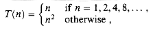
T(n) = aT(n/b) + â(n),
1 and b > 1 be constants, and let â(n) be a nonnegative function defined on exact powers of b. Define T(n) on exact powers of b by the recurrence
(4.6)
T(n) = â(n) + aT(n/b)
= â(n) + aâ(n/b) + a2T(n/b2)
= â(n) + aâ(n/b) + a2â(n/b2) + . . .
+ alogbn-1 f(n/blogbn-1) + alogbnT(1) .
alogbn T(1) =
(nlogba);(1). The remaining terms can be expressed as the sum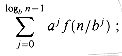
The recursion tree
(1), and each leaf is distance logbn from the root, since n/blogbn = 1. There are alogbn = nlogba leaves in the tree. 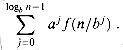 (nlogba).
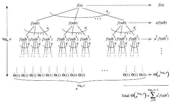
Figure 4.3 The recursion tree generated by T(n) = aT(n/b)+ f(n). The tree is a complete a-ary tree with nlogba leaves and height logb a. The cost of each level is shown at the right, and their sum is given in equation (4.6).
1 and b > 1 be constants, and let â(n) be a nonnegative function defined on exact powers of b. A function g(n) defined over exact powers of b by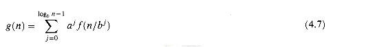
(4.7)
) for some constant > 0, then g(n) = O(nlogba).(nlogba), then g(n) = (nlogba 1g n). câ(n) for some constant c < 1 and all n b, then g(n) = (â(n)).), implying that â(n/bj) = O((n/bj)logba-). Substituting into equation (4.7) yields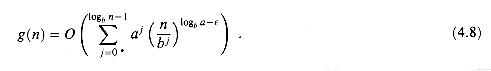
(4.8)
 are constants, the last expression reduces to nlogba-O(n) = O(nlogba). Substituting this expression for the summation in equation (4.8) yields
g(n) = O(nlogba),
(nlogba) for case 2, we have that â(n/bj) = ((n/bj)logba). Substituting into equation (4.7) yields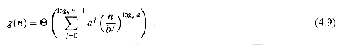
(4.9)
as in case 1, but this time we do not obtain a geometric series. Instead, we discover that every term of the summation is the same: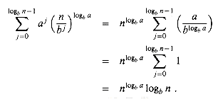
g(n) =
(nlogbalogbn)=
(nlogba 1g n),(n) appears in the definition (4.7) of g(n) and all terms of g(n) are nonnegative, we can conclude that g(n) = ((n)) for exact powers of b. Under the assumption that af (n/b) cf(n) for some constant c < 1 and all n b, we have aj(n/bj) cj (n). Substituting into equation (4.7) and simplifying yields a geometric series, but unlike the series in case 1, this one has decreasing terms: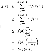 ((n)) for exact powers of b. Case 3 is proved, which completes the proof of the lemma. 1 and b > 1 be constants, and let (n) be a nonnegative function defined on exact powers of b. Define T(n) on exact powers of b by the recurrence
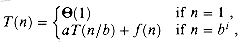 (n) = O(nlogba-) for some constant > 0, then T(n) = (nlogba).(n) = (nlogba), then T(n) = (nlogba lg n).(n) = (nlogba+) for some constant > 0, and if a(n/b) c(n) for some constant c < 1 and all sufficiently large n, then T(n) = ((n)).
T(n) =
(nlogba) + O(nlogba)=
(nlogba),T(n) =
(nlogba) + (nlogba 1g n)=
(nlogba lg n).(n/b) c(n) implies (n) = (nlogba+) (see Exercise 4.4-3). Consequently,T(n) =
(nlogba) + ((n))=
((n)). 4.4.2 Floors and ceilings
T(n) = aT(
n/b) + (n)(4.10)
T(n) = aT(
n/b) + (n)(4.11)
n/b n/b can be pushed through in the first case to yield the desired result, and the bound n/b n/b can be pushed through in the second case. Lower bounding the recurrence (4.11) requires much the same technique as upper bounding the recurrence (4.10), so we shall only present this latter bound. n,
n/b ,n/b/b ,n/b/b/b ,

(4.12)
x x + 1, we obtain
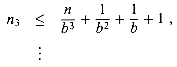
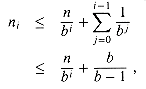 logb n, we obtain ni b + b / (b - 1) = O(1).
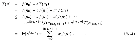
(4.13)

(4.14)
n/b) cf(n) for n > b + b/(b - 1), where c < 1 is a constant, then it follows that aj f(nj) cjf(n). Therefore, the sum in equation (4.14) can be evaluated just as in Lemma 4.3. For case 2, we have f(n) = (nlogba). If we can show that f(nj) = O(nlogba/aj) = O((n/bj)logba), then the proof for case 2 of Lemma 4.3 will go through. Observe that j logbn implies bj/n 1. The bound f(n) = O(nlogba) implies that there exists a constant c > 0 such that for sufficiently large nj, ), which is similar to the corresponding proof of case 2, though the algebra is more intricate.
Exercises
(nlogba 1gk n), where k 0, then the master recurrence has solution T(n) = (nlogba 1gk+1 n). For simplicity, confine your analysis to exact powers of b. cf(n) for some constant c < 1 implies that there exists a constant > 0 such that f(n) = (nlogba+).Problems
2. Make your bounds as tight as possible, and justify your answers. (n/2) + n3.
 (1). (N), where N is the size of the array. (p - q + 1 ) if the subarray A[p . . q] is passed. 2. Make your bounds as tight as possible, and justify your answers.
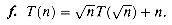 1, b > 1, and f(n) is monotonically increasing. Suppose further that the initial conditions for the recurrence are given by T(n) = g(n) for n n0, where g(n) is monotonically increasing and g(n0) < aT(n0/b)+ f(n0). Prove that T(n) is monotonically increasing.
 as
as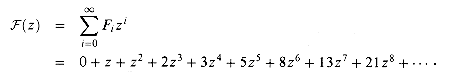
 , rounded to the nearest integer. Hint:
  )
)  i for i 0.
Chip A says Chip B says Conclusion
--------------------------------------------------------
B is good A is good both are good, or both are bad
B is good A is bad at least one is bad
B is bad A is good at least one is bad
B is bad A is bad at least one is bad
n/2 pairwise tests are sufficient to reduce the problem to one of nearly half the size.(n) pairwise tests, assuming that more than n/2 of the chips are good. Give and solve the recurrence that describes the number of tests.Chapter notes