


A tree is a hierarchical collection of nodes. One of the nodes, known as the root, is at the top of the hierarchy. Each node can have at most one link coming into it. The node where the link originates is called the parent node. The root node has no parent. The links leaving a node (any number of links are allowed) point to child nodes. Trees are recursive structures. Each child node is itself the root of a subtree. At the bottom of the tree are leaf nodes, which have no children.
There is a directionality to the links of a tree. In the strictest definition of a tree, the links point down the tree, but never up. In addition, a tree cannot contain cycles. That is, no path originating from a node can return to that node. Figure 10.1(a) shows a set of nodes that have the properties of trees. Figure 10.1(b) shows a set of nodes that do not constitute a tree. That's because node d has two parents, and two cycles are present (a-b-d and a-c-d).
Trees represent a special case of more general structures known as graphs. In a graph, there are no restrictions on the number of links that can enter or leave a node, and cycles may be present in the graph. See the companion volume [Flamig 93] for a discussion of graphs.
Every tree has a height, which is defined as the maximum number of nodes that must be visited on any path from the root to a leaf. For instance, the tree in Figure 10.1(a) has a height of 3. In turn, the depth of a node is the number of nodes along the path from the root to that node. For instance, node c in Figure 10.1(a) has a depth of 1.
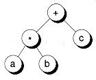
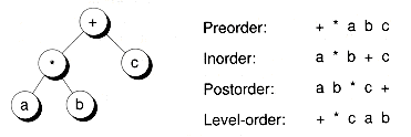
Trees provide a natural way to represent the hierarchical relationship of data. For example, Figure 10.2 shows a tree representing the hierarchical organization of a company. Figure 10.3 shows an example of a tree representing the expression a*b+c. Here, the operators * and + have an order of precedence, where + binds looser than *.
Note In many of the figures in this chapter--including Figures 10.2 and 10.3--the direction of the arrows is implied. Unless otherwise shown, the direction is always from the root downward.
In general, tree nodes can have any number of children. In a binary tree, the nodes have no more than two children. Figures 10.1(a) and 10.3 are examples of binary trees. Figure 10.2 isn't a binary tree because several of its nodes have three children. A node in a binary tree isn't required to have two children. For example, node b in Figure 10.1(a) has only one child. Of course, the leaves of a binary tree have no children.
Binary trees are easy to implement because they have a small, fixed number of child links. Because of this characteristic, binary trees are the most common type of trees and form the basis of many important data structures.
As was true for the linked-list nodes described in Chapter 8, it's useful to define an abstract binary tree node class that doesn't store data, and then derive, using templates, a family of node classes holding different types of data. The following Bnodeb and Bnode classes use this technique:
The Bnodeb and Bnode class definitions are given on disk in the files bnodeb.h and bnode.h.
Many of the binary tree operations are data independent. That's the reason for the Bnodeb class. We can write functions that take Bnodeb pointers as parameters and share these functions across all binary trees, regardless of the type of data actually stored in the nodes. This tames the source code explosion that might otherwise result from the use of templates.
We do pay a price for allowing data independence. When we need to use nodes with data, typecasting problems occur. For instance, the following code fragment will not compile without the typecast shown:
Presumably, all nodes in the tree t store integer data. However, left is typed as a pointer to Bnodeb object, so we need to typecast the expression t->left to be a Bnode<int> pointer. You've seen a similar problem with the linked list nodes described in Chapter 8. The solution is the same: provide convenient functions that hide the typecasting. That's the purpose of Left( ) and Right( ). We can rewrite our code fragment as:
Note carefully that Left( ) and Right( ) actually return references to pointers. This approach allows us to use these functions on the left side of assignments. For instance:
Actually, we don't need to use the Left( ) function in this case, due to the one-way assignment compatibility between derived and base types. For instance, we could write
In the code that follows, we use the pointers left and right directly whenever we can, since the syntax is simpler. We use Left( ) and Right( ) only when necessary. All this typecasting is a bother, but we can't entirely eliminate it and still allow for the use of data-independent code.
The Bnode<TYPE> class has two constructors that are convenient for building trees. The constructors set the left and right pointers to null, unless you specify otherwise. In the following example, we'll build the tree shown in Figure 10.3 :
You'll notice that Bnodeb and Bnode are declared to have all public members. With the linked list nodes described in Chapter 8, we used encapsulation to the fullest, being careful to make all members private when possible. For binary tree nodes, the logistics involved in using fully encapsulated objects get very tedious and messy. For instance, we'll write many standalone functions that operate on Bnodeb pointers--to provide maximum code sharing. While we could make all of these functions friends, and thus make the members of Bnodeb private, it's arguable that little is gained by doing this.
Navigating through trees is at the heart of all tree operations, so it's useful to examine the common issues that arise in tree navigation. The methods we'll show for binary trees can be modified for more general trees.
A tree traversal is a method of visiting every node in the tree. By "visit," we mean that some type of operation is performed. For example, you may wish to print the contents of the nodes. Four basic traversals are commonly used:
1. In a preorder traversal, first the root is visited, then the left subtree, and then the right subtree, recursively.
2. In an inorder traversal, first the left subtree is visited, then the root, and then the right subtree, recursively.
3. In a postorder traversal, first the left subtree is visited, then the right subtree, and then the root, recursively.
4. In a level-order traversal, the nodes are visited level by level, starting from the root, and going from left to right.
Figure 10.4 shows the expression tree presented in Figure 10.3, and the results of traversing the tree using the four types of traversals (where the "visit" function prints node contents). In the context of expression trees, preorder traversal yields what is known as the polish notation for the expression, inorder traversal yields the infix notation (with parenthesis removed, though), and postorder traversal yields the reverse polish notation.
The traversals all have symmetrical cases. For instance, we've defined the traversals to go from left to right. They could alternatively be defined to go right to left, although that is less common in practice.
We'll now explore the first three traversal algorithms, since they can be coded similarly. Level-order traversal will be discussed later.
The first three traversal algorithms are recursive in nature. They must walk down the tree and then back up. Recall, however, that the links of a tree go downward, not upward. Thus, to move back up the tree, each visited parent must be saved for later use. A stack is the natural data structure to use here. As you walk down the tree, parent node pointers can be pushed on the stack. When you go up the tree, these pointers can be popped from the stack. Later, we'll show how to use an explicit stack for this purpose. But first, we'll use the implicit processor stack by writing recursive functions for the traversal algorithms. Here are three such functions, along with a defined type, VisitFunc, which points to a function to be used for the visit action:
The only difference between these functions is the placement of the Visit( ) calls. The placements intuitively suggest the type of traversal that takes place. You'll notice that these functions use generic Bnodeb pointers, and thus they will work for all binary trees. The trick lies in defining the Visit( ) function to work with the type of nodes actually being used. For example, here's how we might set up traversals of the tree given earlier in Figure 10.3 :
Note the typecast in PrtChNode( ). The function must conform to the function pointer type VisitFunc, and thus its parameter must be typed as a Bnodeb pointer. The function assumes, however, that the node is really a Bnode<char> node. All caveats apply for such typecasts.
Since recursion uses processor stack space, it's desirable to eliminate or reduce the recursion as much as possible. In our tree-traversal algorithms, the amount of stack space consumed depends on the height of the tree. That is, for a tree of height n, n parent nodes are placed on the stack. So, for our recursive functions, the recursive calls are up to n levels deep.
Look carefully at the PreOrder( ) and InOrder( ) functions. In these functions, nothing follows the last recursive calls. This type of recursion is known as tail recursion. In a tail-recursive call, the local variables are saved on the processor stack, but they don't really need to be since no action follows the recursive call that needs those variables. Thus, tail recursion can be optimized by eliminating the recursive call and turning it into iteration. For example, here is the PreOrder( ) function written with tail recursion transformed into a while loop. The InOrder( ) function can be coded similarly:
Instead of a call to PreOrder(t->right), t is simply set to t->right and the while loop cycles until a null pointer is found. Note that the recursive call for t->left cannot be eliminated since this call is not tail recursive. Also, no call in PostOrder( ) is tail recursive, so we can't optimize that function any further.
In the recursive calls, the parent node pointer, the Visit function pointer, and the return address are all saved on the processor stack. However, we actually only need to save the parent node pointer. The recursion can thus be optimized by using an explicit stack that saves only node pointers. In doing so, we can also flatten out the recursion and turn it completely into iteration.
The following PreOrderFlat( ) function, modified from the PreOrder( ) function given earlier with tail recursion eliminated, shows the use of an explicit stack:
Here, we've used the ListStk class from Chapter 9, holding pointers to Bnodeb nodes. This stack represents the current path of parents through the tree. Note how the call to PreOrder(t->left) is replaced by a Push( ), followed by the assignment t = t->left. In the original recursive function, the function returns when t is null. This is simulated by doing a Pop( ) from the stack. An InOrderFlat( ) function can be similarly defined. Simply move the Visit( ) call so that it immediately precedes the statement t = t->right.
It's not as easy to turn postorder traversal into iteration because we have no tail recursion to start with. In the PostOrder( ) function, two recursive calls are placed back to back. To use an explicit stack, we must keep track of which recursive call we are in so that we know how to simulate the function return. After the first recursive call, we must pop the parent pointer from the stack and then do another recursive call. After the second recursive call, we must pop the parent from the stack and then visit the node.
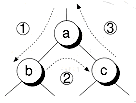
Figure 10.5 shows the three different movements that take place during a post order traversal:
1. Down to the left
2. Up from the left and down to the right
3. Up from the right and then on up the tree.
We can keep track of these movements with a binary state variable. In one state, we're going down the tree. In the other state, we're going up the tree. However, we must clarify whether we're coming up from the left or right. Note that the stack only stores the parent pointer, not which side of the parent we are on. We could store that information as well, but there's a better way. After popping the parent from the stack, we can compare its left or right child pointer to the node we're currently on to determine which side we are coming from. The following PostOrderFlat( ) function utilizes this method:
This function has some further optimizations in it. Notice in state 1 that we inspect the top of the stack (which holds the parent), rather than popping it. With this approach, we don't have to turn around and push the parent back on the stack, in case we need to go down to the right.
The binary tree traversal functions can be found on disk in the file bnodeb.cpp.
At first glance, it appears you would always want to use the flat traversal functions since they use less stack space. But the flat versions aren't necessarily better. For instance, some overhead is associated with the use of an explicit stack, which may negate the savings we gain from storing only node pointers. Use of the implicit function call stack may actually be faster due to special machine instructions that can be used.
The flat traversal functions are useful when the node processing you need to do doesn't depend on where you are in the traversal. Printing the nodes in sequence is one example of this. However, for some tree operations, you must manage more variables than just the nodes themselves. The states of these variables must also be saved on some type of stack. For these operations, using an explicit stack can become more cumbersome than using straightforward recursion. For example, here is a postorder recursive function to find the height of a tree:
The height of a tree is the maximum of the height of its two subtrees. In this case, it's easier to write the function recursively. The flat version is awkward and error prone.
The level-order traversal of a tree (where you go from top to bottom, left to right, level by level) is different from the other traversals because it is not recursive. A queue is needed instead of a stack. The following LvlOrder( ) function shows how the traversal can be accomplished:
In this function, we maintain a queue of nodes to be processed. Nodes are pulled off the queue one at a time, visited, and then the children of the nodes are inserted onto the end of the queue. The net effect is a level order traversal, as shown earlier in Figure 10.4.
One interesting way of performing tree traversals is to use iterator objects. With iterators, it's possible to sequence through a collection of objects at a high level. An iterator is first initialized to point to a particular collection of objects (such as a linked list, array, or tree) and then, using a function such as Next( ), we can ask the iterator to give us the next object in sequence. The iterator object keeps track of the state of the iteration between calls to Next( ). When used on trees, an iterator allows us to "flatten" out a tree and abstract what we mean by "next object."
The following TreeWalkerb class shows how to define an iterator for traversing a binary tree, using any of the four traversal orderings given earlier. This class is written generically using Bnodeb pointers and can thus be shared by all types of binary trees:
Complete code for the TreeWalkerb class is given on disk in the files twalk.h and twalk.cpp. In addition, a derived template class, TreeWalker, is provided to work with specific Bnode<TYPE> trees.
A TreeWalkerb iterator is set up in the constructor by specifying the root of the tree you would like to walk and the traversal order, using the enumerated type WalkOrder. A Reset( ) function does all the work:
An iterator object keeps track of the start of the tree being iterated, in the variable root, plus the node currently being traversed, in the variable curr, plus which traversal function to use in the function pointer variable NextFptr. Note that NextFptr is actually a pointer to a member function, which must be handled differently than ordinary function pointers. See [Stroustrup 91] for more details on member function pointers.
For an iterator object to work, it must keep the state of the iteration between calls to Next( ). Since our traversals our recursive, a stack is needed. For postorder traversals, we also need the binary state variable that indicates whether we're going up or down the tree. In addition, we need a queue for level-order traversals. Rather than use both stack and queue objects, we use a combination staque object instead, which we call path.
The Next( ) function is used to return a pointer to the next node in sequence. Next( ) makes a call to the traversal function pointed to by NextFptr. (Notice the pointer-to-member function call, using the ->* operator.)
Four functions are provided for each type of traversal. These functions are adaptations of the flat-traversal functions given earlier. The difference is that they are member functions and thus have access to the stack stored in the iterator object. Also, instead of making a call to Visit( ), the functions return a pointer to the node to be visited. Before doing the return, though, they must perform actions to ensure that the iterator can pick up where it left off in later calls to Next( ). As an example, here is the NextPreOrder( ) function. You'll notice that it's very similar to the PreOrderFlat( ) function given earlier in the chapter. The other traversal functions can be defined in the same way:
Here is an example of a function that will print out the nodes of a tree using a TreeWalkerb object with all four traversal orders:
A TreeWalkerb iterator has the same problems as the flat-traversal functions. It works great when the nodes can be processed out of context--that is, without regard to where the nodes are in the tree--but it isn't so great when that context must be used in the processing. For example, it's difficult to write the Height( ) function we gave earlier using an iterator. In contrast, it's easy (if somewhat inefficient) to write a function that counts the number of nodes in the tree, as shown in the following function:
When you debug code that works with binary trees, it's useful to print the trees, with the structure of the tree clearly shown. In this section, we'll provide two types of tree printing functions that help in this regard. These functions use the traversal functions given in the previous sections, and they assume very little about the type of screen or printer output available. All that's needed is the C++ iostream object cout to print the nodes line by line.
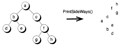
The following PrintSideWays( ) function will print a tree sideways, with the root of the tree on the left and the rightmost node on the first line. Figure 10.6 shows an example.
This function works by using a recursive inorder traversal of the tree. Note, however, that the traversal takes place from right to left, rather than the usual left to right strategy. This means the first node printed is the rightmost node. At each stage in the recursion, we keep track of the number of spaces to print before the node itself is printed. The space variable keeps track of the total (which should start at zero), and inc specifies the spacing to allow between nodes. Since the function is written generically using Bnodeb pointers, the function pointer PrtNode determines the actual function to call in doing the printing. This function is supposed to know the type of data actually stored in the nodes. Here's how PrintSideWays( ) can be called to print the tree given in Figure 10.6 :
While printing sideways is straightforward, the output isn't as easy to use as output that's printed upright. However, upright printing is much harder to do, unless your output device supports random-access positioning. Here, we'll develop a routine that prints a tree upright, line by line.
The key to easy upright printing is to make two passes. The first pass determines the position of each node in the tree. Once the positions are determined, a second pass uses a level-order traversal of the tree to print the nodes line by line.
To keep things simple, we'll assume that each node in the tree is given its own column and that nodes at the same level (that is, having the same depth) are printed on the same line. Thus, the line coordinate (which we'll call y) is equal to the depth of the node. The column, or x coordinate, can be found by the following observation: If you examine the tree shown in Figure 10.7, you'll notice that the node having an x position of one will be the first node visited in an inorder traversal, the node having an x position of two will be the second node visited, and so on.
The following GetNodePosn( ) function uses an inorder traversal to determine the (x, y) positions of each node in a tree. Here, NodeWidth is a pointer to a function that's supposed to return the printing width of a given node:
One major problem lies in finding a place to store the node position information. You could always include (x, y) fields in the nodes themselves. However, that would limit the generality of the function. The GetNodePosn( ) function uses a different technique. It builds an auxilary shadow tree that has the same structure of the tree being traversed. The nodes of this shadow tree keep track of node positions. The node type is given by the following BnodeXY structure, derived from Bnodeb:
After the node positions have been determined, the tree nodes can be printed line by line, using a level-order traversal, with the x position of the nodes determining the spacing between the nodes. The following PrintUp( ) function gives the details:
Note that two level-order iterators are used in PrintUp( ) (the latter uses the TreeWalker template class) to traverse both the main tree and the shadow tree in parallel. You may wonder why we need to store the y position of each node. During a level-order traversal using an iterator, there's no way to tell when we've gone to a new level. Remember that using an iterator loses the shape information of the tree. (In fact, none of the iterative traversals, by themselves, provide enough shape information to reconstruct the tree. See [Lings 86] for more discussion of tree reconstruction.) We detect when a new level has been reached by comparing the y coordinate of the current node with that of the previous node.
Figure 10.8 shows the printed result for the tree shown in Figure 10.7. We used the following code to print the tree:
Complete code for printing a tree sideways and upright is given in the files treeprt.h, treeprt.mth, and treeprt.cpp.
Next, we look at a special class of trees known as binary search trees. A binary search tree has binary nodes and the following additional property: Given a node t, each node to the left is "smaller" than t, and each node to the right is "larger." This definition applies recursively down the left and right subtrees. Figure 10.9 shows a binary search tree where characters are stored in the nodes.
Figure 10.9 also shows what happens if you do an inorder traversal of a binary search tree: you'll get a list of the node contents in sorted order. In fact, that's probably how the name inorder originated.
You may wonder what we mean by "smaller" and "larger" in our definition. This depends on the type of data being stored at the nodes. If, for instance, the data is integers, then the meaning of smaller and larger is obvious. More typically, though, the node data is some kind of structure, with one of the fields (called the key) used to make comparisons. Next, we'll explain how to search a binary tree and how to set up the comparisons for any type of node.
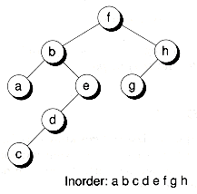
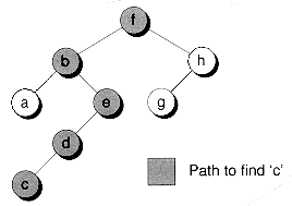
An algorithm for searching a binary search tree follows immediately from the binary search tree property. Although the search algorithm can be cast in a recursive fashion, it's just as easy (and more efficient) to write it iteratively. Here is a Search( ) function that shows how this is done:
Figure 10.10 shows the path taken when searching for a node in a sample tree. The Search( ) function assumes that TYPE has the comparison operators '==' and '<' defined. In the case where TYPE is a built--in type--such as integer or character--this is easy because the operators are already defined. But suppose TYPE is a structure that holds a customer name and a unique integer id. We could use either field as the search key. Here's how you might define the customer structure using the name as the key:
Note that the search string gets converted by the constructor into a Customer object (the Id is given a default value). Obviously, more direct and efficient arrangements are possible. Sometimes, only the key is stored in the nodes, along with a pointer to the actual data. That is also easy to set up. The details are highly application dependent.
Binary search trees provide an efficient way to search through an ordered collection of objects. Consider the alternative of searching an ordered list. The search must proceed sequentially from one end of the list to the other. On average, n/2 nodes must be compared for an ordered list that contains n nodes. In the worst case, all n nodes might need to be compared. For a large collection of objects, this can get very expensive.
The inefficiency is due to the one-dimensionality of a linked list. We would like to have a way to jump into the middle of the list, in order to speed up the search process. In essence, that's what a binary search tree does. It adds a second dimension that allows us to manuever quickly through the nodes. In fact, the longest path we'll ever have to search is equal to the height of the tree. The efficiency of a binary search tree thus depends on the height of the tree. We would like the height to be as small as possible. For a tree holding n nodes, the smallest possible height is logn, so that's how many comparisons are needed on average to search the tree.
To obtain the smallest height, a tree must be balanced, where both the left and right subtrees have approximately the same number of nodes. Also, each node should have as many children as possible, with all levels being full except possibly the last. Searching a well-constructed tree can result in significant savings. For example, it takes an average of 20 comparisons to search through a million nodes! Figure 10.11 shows an example of a well-constructed tree.
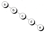
Unfortunately, trees can become so unbalanced that they're no better for searching than linked lists. Such trees are called degenerate trees. Figure 10.12 shows an example. For a degenerate tree, an average of n/2 comparisons are needed, with a worst case of n comparisons--the same cs for a linked list.
When nodes are being added and deleted in a binary search tree, it's difficult to maintain the balance of the tree. We'll investigate methods of balancing trees in the next chapter. In this chapter, we'll use simple tree-construction methods. These methods may result in very unbalanced trees, depending on what order we insert nodes in the tree.
When adding nodes to a binary search tree, we must be careful to maintain the binary search tree property. This can be done by first searching the tree to see whether the key we're about to add is already in the tree. If the key can't be found, a new node is allocated and added at the same location where it would go if the search had been successful. The following Add( ) function shows this technique:
Note that Add( ) calls a function, SearchP( ), to determine where the node should be added. The SearchP( ) function is a modification of Search( ) that returns the parent of the matching node, as well as the matching node itself:
The SearchP( ) function keeps track of which side of the parent the matching node occurs on--in the variable called side. This isn't strictly necessary because we could do an extra compare in Add( ) to determine the side. The following code fragment, taken from Add( ) and modified, shows how:
If the comparison is an expensive operation, it's best to use the side variable instead. Figure 10.13 shows what happens when we use the Add( ) function to add some nodes to a tree.
Deletions from a binary search tree are more involved than insertions. Given a node to delete, we need to consider these three cases:
1. The node is a leaf.
2. The node has only one child.
3. The node has two children.
Case 1 is easy to handle because the node can simply be deleted and the corresponding child pointer of its parent set to null. Figure 10.14 shows an example. Case 2 is almost as easy to manage. Here, the single child can be promoted up the tree to take the place of the deleted node, as shown in Figure 10.15.
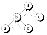
Case 3, where the node to be deleted has two children, is more difficult. We must find some node to take the place of the one deleted and still maintain the binary search tree property. There are two obvious candidates: the inorder predecessor and the successor of the node. We can detach one of these nodes from the tree and insert it where the deleted node used to be. A moment's reflection should convince you that using either of these nodes as the replacement will still maintain the binary search tree property.
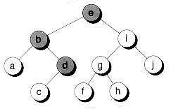
The predecessor of a node can be found by going down to the left once, and then all the way to the right as far as possible. To find the successor, an opposite traversal is used: first to the right, and then down to the left as far as possible. Figure 10.16 shows the path taken to find both the predecessor and successor of a node in a sample tree.
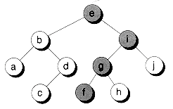
Both the predecessor and successor nodes are guaranteed to have no more than one child, and they may have none. (Think about how the traversals take place: they always end when the corresponding left or right child is null.) Because of this, detaching the predecessor or successor reduces to either Case 1 or 2, both of which are easy to handle. In Figure 10.17, we delete a node from the tree and use its successor as the replacement.
For the replacement, many texts suggest that you copy the data of the replacement node into the node that would have been detached, and then detach the replacement. However, if the node data is large, this involves a lot of data movement. In fact, it defeats one of the reasons for using a non-contiguous data structure! We'll perform the replacement by leaving the node data where it is, and use pointer surgery instead. That's the approach taken by the following DetachNode( ) function. This function is written generically using Bnodeb pointers, reinforcing the fact that no data is actually moved:
The DetachNode( ) function uses the following ParentOfSuccessor( ) function to find the parent of the successor node. We want the parent so that we can easily detach the successor from its original location:
Both DetachNode( ) and ParentOfSuccessor( ) can be written generically with Bnodeb pointers. We don't need to do any key comparisons since the structure of the tree lets us find the nodes we're looking for.
The DetachNode( ) function is called by higher-level functions that determine which node to detach. For example, here's a Detach( ) function that first searches for a node having matching data to x, and then proceeds to detach that node:
Finally, to actually deallocate the node, we use the following Delete( ) function:
Deleting all the nodes from a tree can be done recursively, using a postorder traversal. The following Clear( ) function clears a tree by calling a recursive DelTree( ) function:
By using postorder traversal, the nodes are deleted from the bottom up. Note that it would be difficult to use any other type of traversal here because we would have to delete nodes before we're through with them. The DelTree( ) function can alternatively be written non-recursively, using a postorder iterator object:
To copy a tree, you must first clear the destination tree and then duplicate the nodes of the source tree. The following Copy( ) function calls the Clear( ) function and then calls a recursive DupTree( ) function to do the node duplication. The latter function uses postorder traversal to build the duplicate tree from the bottom up:
Here's an interesting twist to the technique for copying trees: Use an iterator object on the source tree, traverse the tree in some order, and insert duplicated nodes into the destination tree by using the Add( ) function. The following alternative Copy( ) function does this:
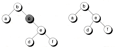
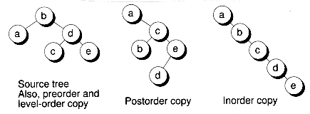
Figure 10.18 shows the results when we use the four different types of traversals on the source tree during copying. Notice that both preorder and level-order traversals produce a destination tree that has the same structure as the source tree. A postorder traversal yields a different structure, but it's still a valid binary search tree.
As you can see, the order that you insert nodes into a binary search tree does make a difference. In fact, if you insert nodes into a tree in sorted order, as exemplified by the inorder traversal copying in Figure 10.18, the result is a degenerate tree. This fact suggests you should avoid inserting nodes into a binary search tree in sorted order. In the next chapter, we'll look at ways of circumventing this problem.
You'll notice that operations like Add( ) and Delete( ) are awkward due to the unidirectional capability of the links. We must write the operations in terms of finding the parent of a desired node, rather than find the node directly. This problem is similar to those we had with singly-linked lists in Chapter 8. The clumsiness can be alleviated by adding an extra pointer in each node, which points to the parent of the node. The result is known as a threaded binary tree. Figure 10.19 shows an example. A threaded tree is to a normal tree what a doubly-linked list is to a singly-linked list--it allows easy traversal in both directions. Note that, in a strict sense, a threaded binary tree isn't a true tree because it has cycles.
By using a threaded binary tree, it's possible to write the tree-traversal routines without recursion and without a stack. Since a stack isn't needed, tree operations can be faster, due to reduced overhead. However, before you try to reimplement all the algorithms you've seen in this chapter, keep in mind that the price you pay is space overhead in the tree nodes. (This is the same speed vs. space tradeoff you've seen repeatedly.) You pay for the overhead of parent pointers with every node, regardless of whether you need those pointers. When you use a stack, you pay for the overhead of the stack only when needed, and that overhead grows with the height of the tree, not with the number of nodes in the tree.
We're not recommending that you avoid using parent pointers, only that you be sure to consider the tradeoffs. Code without parent pointers is only slightly more complicated than code with them. After the operations are coded, the fact that they may be a little clumsly becomes a moot point. For maximum speed, however, you may want to use parent pointers.
As a final note, we should tell you that you can implement other forms of threaded trees. For example, one particular type uses extra pointers that allow you to directly find the next and previous nodes assuming an inorder traversal. See [Horosahni 90] for details.
We've used standalone functions to implement the basic binary tree operations. However, it might be useful to encapsulate these into a class and to make binary trees look like concrete data types. The following Bstree class shows an example:
Complete code for the Bstree class is given on disk in the files bstree.h, bstree.mth, and bstreeb.cpp. A test program is provided in tstbs.cpr. This program uses the tree-walking and tree printing functions given earlier in the chapter.
A Bstree object serves as a handle to a binary tree. Stored in each Bstree object is a pointer, root, to the top node of the tree. Many of the functions we gave earlier passed the root of the tree as the first argument. These functions can be adapted for the Bstree class by removing the first argument, and relying instead on the implicit this pointer that's passed. For example, here's the new Add( ) function:
The Bstree class is set up like most the concrete data type classes in this book--with ample constructors, destructors, overloaded assignment operators, and so on. Whether or not you need all these functions is, of course, up to you. We've added some functions that retrieve and delete the minimum and maximum nodes from the tree. The minimum node can be found by going left as far as possible. The maximum node can be found by going right as far as possible.
Similar to the linked-list classes defined in Chapter 8, we've provided the virtual functions AllocNode( ) and FreeNode( ), which you can override to change how the tree nodes are allocated. For example, a binary tree can be stored contiguously using an array of nodes, as well as on the heap with non-contiguous nodes.
A few hints for building trees with arrays: You'll want to maintain a singly-linked free list of deleted tree nodes. This can be done by reusing the left (or, alternatively, right) child pointers to serve as the free list's next pointers. Also, nothing prevents you from dispensing with pointers altogether and instead using two parallel arrays of indexes that correspond to the left and right child links.
If you don't plan on overriding AllocNode( ) and FreeNode( ), you can declare them as static, along with the recursive functions DupTree( ) and DelTree( ). This will result in more efficient code, since in the recursive function calls, the implicit this pointer won't be passed.
Figure 10.1 A tree and a non-tree.
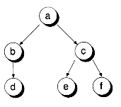
(a) A tree
(b) Not a tree
Figure 10.2 An organization tree for a typical company.
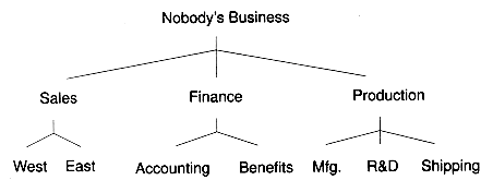
Figure 10.3 An expression tree.
Binary Trees
Binary Tree Node Classes
struct Bnodeb { // An abstract binary tree nodeBnodeb *left; // Pointer to left child
Bnodeb *right; // Pointer to right child
};
template<class TYPE>
struct Bnode : public Bnodeb { // Binary tree node with dataTYPE info;
Bnode();
Bnode(const TYPE &x, Bnode<TYPE> *l=0, Bnode<TYPE> *r=0);
Bnode<TYPE> *&Left();
Bnode<TYPE> *&Right();
} ;
template<class TYPE>
Bnode<TYPE>::Bnode()
{left = 0; right = 0;
}
template<class TYPE>
Bnode<TYPE>::Bnode(const TYPE &x, Bnode<TYPE> *l, Bnode<TYPE> *r)
: info(x)
{left = l; right = r;
}
template<class TYPE>
Bnode<TYPE> *&Bnode<TYPE>::Left()
{return (Bnode<TYPE> *)left;
}
template<class TYPE>
Bnode<TYPE> *&Bnode<TYPE>::Right()
{return (Bnode<TYPE> *)right;
}

Bnode<int> *t;
...
t = (Bnode<int> *)(t->left); // Base to derived typecast
Bnode<int> *t;
...
t = t->Left();
Bnode<int> *t, *p;
...
t->Left() = p;
Bnode<int> *t, *p;
...
t->left = p; // Implicit derived to base typecast
Bnode<char> a('a'), b('b'), c('c');Bnode<char> times('*', &a, &b);Bnode<char> plus('+', ×, &c); TREE TRAVERSALS
Recursive Traversals
Figure 10.4 The four tree traversals.
typedef void (*VisitFunc) (Bnodeb *n);
void PreOrder(Bnodeb *t, VisitFunc Visit)
{if (t) {Visit(t);
PreOrder(t->left, Visit);
PreOrder(t->right, Visit);
}
}
void InOrder(Bnodeb *t, VisitFunc Visit)
{if (t) {InOrder(t->left, Visit);
Visit(t);
InOrder(t->right, Visit);
}
}
void PostOrder(Bnodeb *t, VisitFunc Visit)
{if (t) {PostOrder(t->left, Visit);
PostOrder(t->right, Visit);
Visit(t);
}
}
void PrtChNode(Bnodeb *b)
{cout << ((Bnode<char> *)b)->info << ' ';
}
Bnode<char> a('a'), b('b'), c('c');Bnode<char> times('*', &a, &b);Bnode<char> plus('+', ×, &c);PreOrder(&plus, PrtChNode); cout << '\n';
InOrder(&plus, PrtChNode); cout << '\n';
PostOrder(&plus, PrtChNode); cout << '\n';
Eliminating Tail Recursion
void PreOrder(Bnodeb *t, VisitFunc Visit)
// Tail recursion eliminated
{while(t) {Visit(t);
PreOrder(t->left, Visit);
t = t->right;
}
}
Flattening out Recursion
void PreOrderFlat(Bnodeb *t, VisitFunc Visit)
{ListStk<Bnodeb *> path;
while(1) {if (t) {Visit(t);
// Simulate call PreOrderFlat(t->left, Visit);
path.Push(t);
t = t->left;
}
else {// Simulate function return
if (path.Pop(t) == 0) break;
// Optimize the tail recursion
t = t->right;
}
}
}
void PostOrderFlat(Bnodeb *t, VisitFunc Visit)
{ListStk<Bnodeb *> path;
int state = 0;
while(1) {if (state == 0) {// Ready to go down to the left
if (t) {path.Push(t);
t = t->left;
}
else state = 1;
}
else { // State 1: Ready to come up from either directionBnodeb *c = t;
if (path.IsEmpty ()) break;
t = *path.Top();
if (c == t->left && t->right) {// Coming back up the tree from the left, and
// since there is a right child, go right.
// Note that t is still on top of stack.
t = t->right;
state = 0;
}
else {// Coming back up the tree from the right,
// or there was no right child, so visit
// the node and continue on up. (State
// stays at 1.)
Visit(t);
path.Pop( );
}
}
}
}
Figure 10.5 The three movements in a traversal.

To Recurse or Not to Recurse
int Height(Bnodeb *t)
{int h = 0;
if (t != 0) {int lh = Height(t- >left);
int rh = Height(t- >right);
h = ((lh > rh) ? lh : rh) + 1;
}
return h;
}
Level-Order Traversal
void LvlOrder(Bnodeb *t, VisitFunc Visit)
}
ListQ<Bnodeb *> nodes_left;
nodes_left.Insert(t);
while(1) {Bnodeb *p;
if (nodes_left.Extract(p) == 0) break;
Visit(p);
if (p->left != 0) nodes_left.Insert(p->left);
if (p->right != 0) nodes_left.Insert(p->right);
}
}
TREE WALKING ITERATORS
enum WalkOrder { pre_order, post_order, in_order, lvl_order };class TreeWalkerb { // Tree-walking base classprotected:
ListSQ<Bnodeb *> path;
Bnodeb *root, *curr;
WalkOrder worder;
int state;
Bnodeb *NextPreOrder();
Bnodeb *NextInOrder();
Bnodeb *NextPostOrder();
Bnodeb *NextLvlOrder();
Bnodeb *(TreeWalkerb::* NextFptr)();
public:
TreeWalkerb(Bnodeb *r, WalkOrder w);
virtual ~TreeWalkerb();
void Reset();
void Reset(Bnodeb *r, WalkOrder w);
Bnodeb *Next ();
};

TreeWalkerb: :TreeWalkerb(Bnodeb *r, WalkOrder w)
{Reset( r, w);
}
void TreeWalkerb::Reset(Bnodeb *r, WalkOrder w)
{root = r;
worder = w;
if (worder == pre_order) NextFptr = &TreeWalkerb: :NextPreOrder;
else if (worder == in_order) NextFptr = &TreeWalkerb: :NextInOrder;
else if (worder == post_order) NextFptr = &TreeWalkerb: :NextPostOrder;
else NextFptr = &TreeWalkerb: :NextLvlOrder;
state = 0; curr = root;
path.Clear();
if (root && worder == lvl_order) path.Insert(root);
}
Bnodeb *TreeWalkerb: :Next()
{return (this->*NextFptr)();
}
Bnodeb *TreeWalkerb::NextPreOrder()
{while(1) {if (curr) {path.Push(curr);
Bnodeb *p = curr;
curr = curr->left; // Set up for next visit
return p; // So the node can be "visited"
}
else {if (path.Pop(curr) == 0) {return curr = 0; // Signal no more nodes
}
else curr = curr->right;
}
}
}
void PrintNode(Bnodeb *t)
// Assumes node is actually a Bnode<char> node
{cout << ((Bnode<char> *)t)->info << '\n';
}
void PrintTreeOrderings(Bnode<char> *root)
{Bnodeb *nxt;
if (root == 0) { cout << "Tree is empty\n"; return; }cout << "PreOrder: ";
TreeWalkerb tw(root, pre_order);
while((nxt = tw.Next()) != 0) PrintNode(nxt);
cout << '\n';
cout << "InOrder: ";
tw.Reset(root, in_order);
while((nxt = tw.Next()) != 0) PrintNode(nxt);
cout << '\n';
cout << "PostOrder: ";
tw.Reset(root, post_order);
while((nxt = tw.Next()) != 0) PrintNode(nxt);
cout << '\n';
cout << "Level Order: ";
tw.Reset(root, lvl_order);
while((nxt = tw.Next()) != 0) PrintNode(nxt);
cout << '\n';
}
int NumNodes(Bnodeb *t)
// Determine number of nodes in the tree t
{Bnodeb *nxt;
int cnt = 0;
TreeWalkerb tw(t, in_order); // Any ordering will do
while((nxt = tw.Next()) != 0) cnt++;
return cnt;
}
PRINTING TREES
Printing Sideways
Figure 10.6 A tree printed sideways.
typedef void (*PrtFunc)(Bnodeb *n);
void PrintSideWays(Bnodeb *t, PrtFunc PrtNode, int inc, int space)
{while(t) {PrintSideWays(t->right, PrtNode, inc, space+inc);
for(int i = 0; i<space; i++) cout << ' ';
PrtNode(t); cout << '\n';
t = t->left;
space += inc;
}
}
void PrtChNode(Bnodeb *t) { cout << ((Bnode<char> *)t)->info; }Bnode<char> *t;
... // Set up t to be the tree in Figure 10.6
PrintSideWays(t, PrtChNode, 3, 0);
Printing Upright
typedef int (*NodeWidthFunc)(Bnodeb *n);
BnodeXY *GetNodePosn(Bnodeb *t, int &x, int y, NodeWidthFunc NodeWidth)
// Using an inorder traversal, figure out x and y of each node
// in the tree t, assuming that the top left corner of the
// box bounding t is at (x, y). Builds a parallel shadow tree
// of nodes having x and y in them.
{if (t == 0) return 0;
BnodeXY *l = GetNodePosn(t->left, x, y+1, NodeWidth);
BnodeXY *xyt = new BnodeXY;
xyt->left = l;
xyt->x = x;
x += NodeWidth(t);
xyt->y = y;
y++;
xyt->right = GetNodePosn(t->right, x, y, NodeWidth);
return xyt;
}
Figure 10.7. A row- and column-aligned tree.
struct BnodeXY : public Bnodeb {int x, y;
BnodeXY *Left( ) { return (BnodeXY *) left; }BnodeXY *Right( ) { return (BnodeXY *) right; }} ;
void PrintUp(Bnodeb *t, PrtFunc PrtNode, NodeWidthFunc NodeWidth)
{int spacing, last_sp, x, oldy;
Bnodeb *nxt;
BnodeXY *xynxt;
if (t == 0) { cout << "Empty tree\n"; return; }x = 1;
BnodeXY *xyt = GetNodePosn(t, x, 0, NodeWidth);
TreeWalkerb tw(t, lvl_order);
TreeWalker<BnodeXY> xytw(xyt, lvl_order);
oldy = 0;
last_sp = 0;
while(1) {xynxt = xytw.Next();
if (xynxt == 0) break;
if (xynxt->y != oldy) {oldy = xynxt->y;
cout << '\n';
last_sp = 0;
}
spacing = xynxt->x - last_sp - 1;
if (spacing < 0) spacing = 0;
while(spacing-) cout << ' ';
nxt = tw.Next();
PrtNode(nxt);
last_sp = xynxt->x + NodeWidth(nxt) - 1;
}
cout << "\n\n";
// Need to delete shadow tree. Easy to do with postorder traversal
xytw.Reset(xyt, post_order);
while(1) {xynxt = xytw.Next();
if (xynxt == 0) break;
delete xynxt;
}
}
void PrtChNode(Bnodeb *t)
{cout << ((Bnode<char> *)t)->info;
}
int ChNodeWidth(Bnodeb *t)
{return 1; // This is the printing width
}
Bnode<char> *t;
// Build tree in Figure 10.7
...
PrintUp(t, PrtChNode, ChNodeWidth);

BINARY SEARCH TREES
Binary Tree Searching
Figure 10.8 A tree printed upright.

Figure 10.9 A binary search tree.
template<class TYPE>
Bnode<TYPE> *Search(Bnode<TYPE> *t, const TYPE &x)
// Returns pointer to a node matching the data x if
// such a node is in the tree t; otherwise, a 0 is returned
{while (t) {if (x == t->info) break;
t = (x < t->info) ? t->Left() : t->Right();
}
return t;
}
struct Customer {char name[80];
int id;
Customer(char *n, int i = 0; // Notice default argument
};
Customer::Customer(char *n, int i)
{strncpy(name, n, 80);
name[79] = 0; // Ensure null termination
Id = i;
}
int operator==(Customer &a, Customer &b)
{return !strcmp(a.name, b.name);
}
int operator<(Customer &a, Customer &b)
{return strcmp(a.name, b.name) < 0;
}
... // Other operators similarly defined
Bnode<Customer> *custdb;
...// Build the tree, then search it
if (Search(custdb, "Ford Prefect")) cout << "Customer found\n";
Figure 10.10 Searching a binary tree.
Why Use Binary Search Trees?
Figure 10.11 A well-constructed binary search tree.
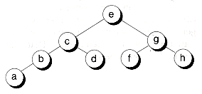
Figure 10.12 A degenerate binary search tree.
Inserting Nodes into a Binary Search Tree
template<class TYPE>
Bnode<TYPE> *Add(Bnode<TYPE> *&root, const TYPE &x, int &exists)
// Returns matching node, new or old. May modify the root pointer.
{Bnode<TYPE> *p;
int side;
// Look for a place to insert the node
Bnode<TYPE> *t = SearchP(root, x, p, side);
if (t == 0) { // No matching node foundt = new Bnode<TYPE>(x); // left and right should be set to 0
if (p) {if (side) p->right = t; else p->left = t;
}
else root = t; // No parent, so we have a new root
existed = 0;
}
else existed = 1;
return t;
}
template<class TYPE>
Bnode<TYPE> *
SearchP(Bnode<TYPE> *t, const TYPE &x, Bnode<TYPE> *&p, int &side)
// Returns matching node in tree t, along with parent. If
// matching node is t itself, a 0 is passed back for the parent.
// Returns 0 if no match found.
{p = 0;
while (t) {if (x == t->info) break;
p = t;
if (x < t->info) {side = 0;
t = t->Left();
}
else {side = 1;
t = t->Right();
}
}
return t;
}
if (p) {// Used to be: if (side) p->right = t; else p->left = t;
if (p->info < x) p->right = t; else p->left = t;
}
Figure 10.13 Inserting nodes into a binary search tree.

Deleting Nodes from a Binary Search Tree
Figure 10.14 Deleting a leaf node.

Figure 10.15 Deleting a node that has one child.
Bnodeb *DetachNode(Bnodeb *&root, Bnodeb *t, Bnodeb *p, int side)
// Detaches node t with parent p from the tree. Node t is
// the left child if side = 0; otherwise, it's the right child.
// If p is 0, then it is the root, and that is handled
// accordingly. Redundantly returns the pointer t. May
// have to update root pointer.
{Bnodeb *psucc, *replacement;
if (t) {if (t->left == 0 || t->right == 0) {// At least one child is null, so use the other
// as the replacement. (It may be null, too.)
replacement = (t->left) ? t->left : t->right;
}
else { // Neither child is nullpsucc = ParentOfSuccessor(t); // Guaranteed not null
if (psucc == t) { // Immediate successorreplacement = psucc->right;
}
else {// Detach replacement from its current location
// and relocate it to where t used to be
replacement = psucc->left;
psucc->left = psucc->left->right;
replacement->right = t->right;
}
// Finish relocating replacement to go where t used to be
replacement->left = t->left;
}
if (p) { // Fix parent of t to point to replacementif (side)
p->right = replacement; else p->left = replacement;
}
else root = replacement; // No parent, so t was the root
}
return t;
}
Figure 10.16 Finding predecessor and successor nodes.
(a) Predecessor of 'e'
(b) Successor of 'e'
Figure 10.17 Deleting a node that has two children.

(a) Before deleting 'e'
(b) After deleting 'e'
Bnodeb *ParentOfSuccessor(Bnodeb *t)
// If no successor, a 0 is returned
{Bnodeb *p = 0;
// Go right, then all the way left
Bnodeb *q = t->right;
if (q) {p = t;
while(q->left) {p = q;
q = q->left;
}
}
return p;
}
template<class TYPE>
Bnode<TYPE> *Detach(Bnode<TYPE> *&root, const TYPE &x)
// Detaches node matching x from the tree.
// May have to update the root pointer.
{int side;
Bnode<TYPE> *p, *t;
t = SearchP(root, x, p, side);
return (Bnode<TYPE> *)DetachNode((Bnodeb *)root, t, p, side);
}
template<class TYPE>
int Delete(Bnode<TYPE> *&root, const TYPE &x)
// Returns 1 if node actually found; otherwise, returns 0
// May have to update the root pointer
{Bnode<TYPE> *n = Detach(root, x);
delete n;
return n != 0;
}
Clearing and Copying Binary Trees
template<class TYPE>
void Clear(Bnode<TYPE> *&root)
{DelTree(root);
root = 0;
}
template<class TYPE>
void DelTree(Bnode<TYPE> *t)
{if (t == 0) return;
DelTree(t->Left());
DelTree(t->Right());
delete t;
}
template<class TYPE>
void Bstree<TYPE>::DelTree(Bnode<TYPE> *t)
{TreeWalker< Bnode<TYPE> > tw(t, postorder);
Bnode<TYPE> *nxt;
while((nxt = tw.Next()) != 0) delete nxt;
}
template<class TYPE>
int Copy(Bnode<TYPE> *&root, const Bstree<TYPE> &t)
{Clear(root);
Bnode<TYPE> *r = DupTree(t.root);
if (r) {root = r;
return 1; // Success
}
else return 0; // Failure
}
template<class TYPE>
Bnode<TYPE> *DupTree(Bnode<TYPE> *t)
{if (t == 0) return 0;
Bnode<TYPE> *l = DupTree(t->Left());
Bnode<TYPE> *r = DupTree(t->Right());
return new Bnode<TYPE>(t->info, 1, r);
}
template<class TYPE>
int Copy(Bnode<TYPE> *&root, const Bstree<TYPE> &t, WalkOrder w)
{Clear(root);
TreeWalker< Bnode<TYPE> > tw(t.root, w);
Bnode<TYPE> *nxt;
int dmy;
while((nxt = tw.Next()) != 0) Add(root, nxt->info, dmy);
return 1;
}
Figure 10.18 Copying via source tree traversals.
THREADED BINARY TREES
Figure 10.19 A threaded binary tree.
BINARY TREES AS CONCRETE DATA TYPES
template<class TYPE>
class Bstree { // A binary tree of nodes holding TYPE dataprotected:
Bnode<TYPE> *root;
Bnode<TYPE> *SearchP(const TYPE &x, Bnode<TYPE> *&p, int &side);
virtual Bnode<TYPE> *AllocNode
(const TYPE &x, Bnode<TYPE> *1=0, Bnode<TYPE> *r=0);
Bnode<TYPE> *DupTree(Bnode<TYPE> *t);
virtual void FreeNode(Bnode<TYPE> *n);
void DelTree(Bnode<TYPE> *t);
public:
Bstree();
Bstree(const Bstree<TYPE> &t);
virtual ~Bstree();
void operator=(const Bstree<TYPE> &t);
int Copy(const Bstree<TYPE> &t);
int Copy(const Bstree<TYPE> &t, WalkOrder w);
void Clear();
Bnode<TYPE> *Member(const TYPE &x);
const Bnode<TYPE> *Member(const TYPE &x) const;
Bnode<TYPE> *Add(const TYPE &x, int &existed);
Bnode<TYPE> *Add(const TYPE &x);
Bnode<TYPE> *Detach(const TYPE &x);
Bnode<TYPE> *DetachMin();
Bnode<TYPE> *DetachMax();
int Delete(const TYPE &x);
void DeleteMin();
void DeleteMax();
Bnode<TYPE> *Root();
Bnode<TYPE> *Min();
Bnode<TYPE> *Max();
int IsEmpty() const;
};

template<class TYPE>
Bnode<TYPE> *Bstree<TYPE>::Add(const TYPE &x, int &exists)
{Bnode<TYPE> *p;
int side;
Bnode<TYPE> *t = SearchP(x, p, side);
if (t == 0) {t = AllocNode(x);
if (p) {if (side) p->right = t; else p->left = t;
}
else root = t;
existed = 0;
}
else existed = 1;
return t;
}
SUMMARY