12.5.3 Implementation

Just as in the Huffman tree construction, if we are not careful we will end up with an O(n²) time implementation. Instead, we can use a heap similar to that for the Huffman construction to obtain an O(n 1g n) time requirement and O(n) storage. However, we can do even better.

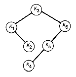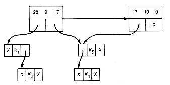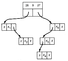
Figure 12.15 Greedy Binary Search Tree Constructed as Illustrated in Figure 12.14

The preceding method leads to a sequence of n - 1 combined triples with values v₁, v₂, . . . , v_n-1. In this sequence v₁ ?/FONT> v₂ ?/FONT> . . . ?/FONT> v_n-1. That is, the triples are generated in order, from the smallest to the highest value. The improved algorithm, introduced now, also generates a sequence of n - 1 combined triples, but their values will not necessarily be the same as v₁, . . . , v₂, v_n-1, nor will they necessarily be generated in order by size. The improved algorithm, however, will produce the greedy tree that would have been obtained had they been combined in order by size when it is unique. A unique tree exists when there is exactly one smallest triple at each step. In general, the resultant tree will be greedy, but it will not necessarily be the same greedy tree generated by v₁, . . . , v₂, v_n-1, nor will it necessarily have the same weighted path length.

We start with a list-structure illustrated in Figure 12.16. Each record represents a potential triple to be combined in the construction of a greedy tree. Traverse the list starting at the left and search for a locally minimal triple -- that is, a triple whose value does not exceed the value of its successor triple. No triple to the left of this locally minimal triple can be combined before it in any greedy tree construction. In addition, any future combining of locally minimal triples to its right cannot cause the resultant tree to fail to be greedy. In other words, combining the minimal triple always allows a greedy tree to be constructed with the combined minimal triple as a subtree. Combine the locally minimal triple (say it is the ith), and obtain the new list-structure shown in Figure 12.16(b).

Here a?/FONT>_i-1 and a?/FONT>_i were both set to the value of the combined triple a?/FONT>_i?SUB>1 + b_i + a?/FONT>_i, the ith record was deleted, and the pointers changed as shown. The left-to-right traversal is continued, starting now at the (i - 2)th record, combining as before for each locally minimal triple encountered. Details involving the ends of the list-structure can be handled by special checking or by introducing artificial records with large weights at the ends. This results in the construction of a greedy tree. This procedure is reminiscent of the evaluation of an infix expression of Chapter 4. That algorithm is greedy in the sense that we look for the highest local priority operator to evaluate first in a left-to-right scan, evaluate it, and continue from that point.

(a) Starting List Structure

(b) List Structure after Combining the ith Locally Minimal Triple

(c) Starting List Structure for the Weights of Example 12.3

(d) Result of Combining the Triple 6 3 4

(e) Result of Combining 4 2 3

(f) Result of Combining 5 10 13

(g) Result of Combining 9 0 8

(h) Result of Combining 17 10 0

(i) Result of Combining 28 9 27

Figure 12.16 Implementation of the Greedy Algorithm

Applying this improved algorithm to Example 12.3, the starting list-structure is as shown in Figure 12.16(c). The first locally minimal triple found is 6 3 4. The list-structure resulting from combining it is shown in Figure 12.16(d). Starting again at the first record, 4 2 3 is the next minimal triple, yielding the list shown in Figure 12.16(e). Starting again, the first record here is found to be the locally minimal triple to obtain the list shown in Figure 12.16(f).

Starting again at the next first record, 9 0 8, the next locally minimal triple, gives the list shown in Figure 12.16(g). Once again, we start at the first record. The next locally minimal triple is 17 10 0. Combining it results in Figure 12.16(h). Finally the triple 28 9 27 is combined to obtain the result shown in Figure 12.16(i).

We have constructed the same tree as before (in Figures 12.14 and 12.15). Again, this need not always occur. However, even when it does, as here, the order in which the subtrees were formed need not be the same. We generated subtrees with values 13, 9, 28, 17, 27, and finally 64, rather than in order from the smallest to largest as in the other method. Both trees in this example have the same weighted path length of 188.

This implementation takes time and storage only O(n)! This was made possible by the new method, coupled with the proper choice of data structure.